SWI Prolog: SWI Prolog is computer software that is used to run programs written in Prolog language. It is developed by Jan Wielemaker. It is free software written in C language and can be run on different platforms like Linux, Unix, windows, mac, etc. SWI stands for Social-Wetenschappelijke Informatica which means “Social Science Informatics”, it is actually the name of group at University of Amsterdam where Jan Wielemaker worked as an employee. Its initial release was in 1987 and its first stable release was in 2021. In this software facts for any logical program can be written using conditional representation and after the compilation, the program can be tested for success or failure.
Prolog : Prolog is considered as a declarative language rather than programming language as it is not used to solve computational problems. It is used to solve logical problems which use rules or facts. The full form of prolog is programming in logic. Prolog is used in much artificial intelligence, natural language processing, and machine learning problems. Prolog is used to write facts or rules for problems and then prolog’s run time system checks those facts and rules whenever that problem is asked and returns a true or false statement for success or failure of the problem.
Installing SWI Prolog onWindows:
Follow the below steps to install SWI Prolog on Windows:
Step 1: Visit swi-prolog.org website using any web browser.

Step 2: Click on Download which is adjacent to Home, dropdown list will appear then click on SWI-Prolog.

Step 3: New webpage will open, click on Stable release.

Step 4: After clicking on stable release new webpage will open which will contain stable versions of prolog for different platforms. Under binaries there are two stable releases for windows, first is SWI-Prolog 8.4.0-1 for Microsoft Windows (64 bit) and the other is SWI-Prolog 8.4.0-1 for Microsoft Windows (32 bit). Click on the one as per your system configuration. Lets take the one for 64-bit operating system.

Step 5. After clicking on SWI-Prolog 8.4.0-1 for Microsoft Windows (64 bit), a new webpage will open, check on I understand checkbox to make the download link active. Then click on the download link, downloading of the executable file will start shortly. It is a small 11.9 MB file that will hardly take a minute.

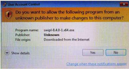
Step 6: Now check for the executable file in downloads in your system and run it.

Step 7: It will prompt confirmation to make changes to your system. Click on Yes.
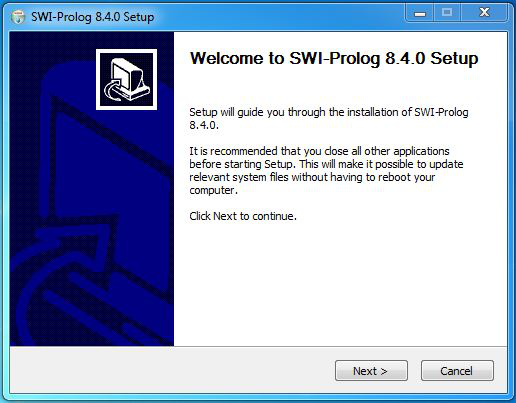
Step 8: Setup screen will appear, click on Next.
Step 9: The next screen will be of License Agreement, click on I Agree.

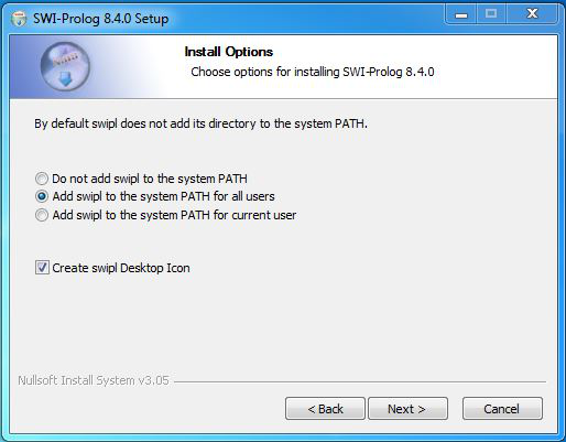
Step 10: After it there will be screen of installing options so check the box for Add swipl to the system path for all users, and also check the box for create a desktop icon and then click on the Next button.
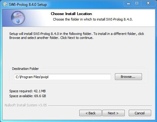
Step 11: The next screen will be of installing location so choose the drive which will have sufficient memory space for installation. It needed only a memory space of 50 MB.
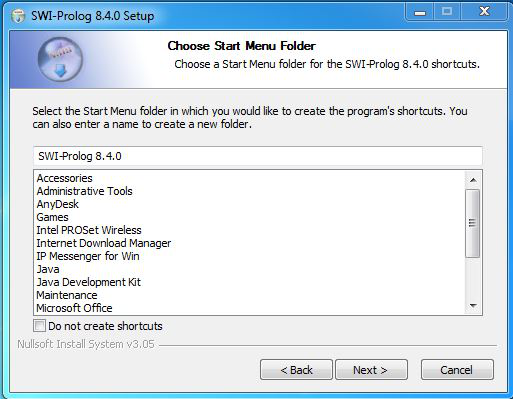
Step 12: Next screen will be of choosing Start menu folder so don’t do anything just click on Next Button.
Step 13: This last screen is of choosing components, all components are already marked so don’t change anything just click on Install button.

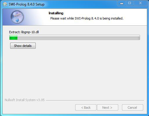
Step 14: After this installation process will start and will hardly take a minute to complete the installation.
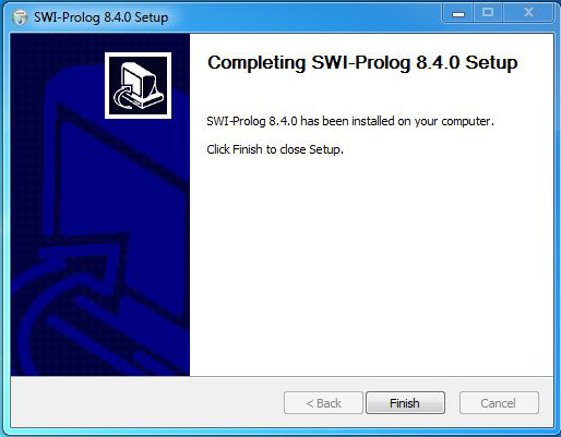
Step 15: Click on Finish after the installation process is complete.
Step 16: SWI Prolog is successfully installed on the system and an icon is created on the desktop.

Step 17: Run the software and see the interface.
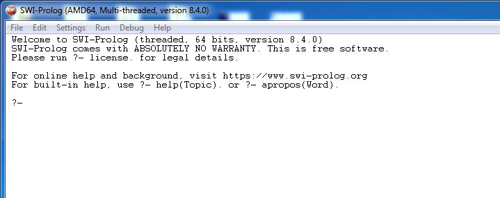
Congratulations!! At this point, you have successfully installed SWI-Prolog on your windows system.
1 2 3 4 5 6 7 8 9 10 11 12 13 14 15 16 17 18 19 20 21 22 23 24 25 26 27 28 29 30 31 32 33 34 35 36 37 38 39 40 41 42 43 44 45 46 47 48 49 50 51 52 53 54 55 56 57 58 59 |
implement main open core, console /* Программа: Служащие */ /* Назначение: Демонстрация использования селектирующих правил на основе ОПН-метода (откат после неудачи)*/ domains name = symbol. sex = symbol. department = symbol. pay_rate = real. class predicates employee : (name,sex,department,pay_rate) nondeterm anyflow. show_part_time : (). show_male_part_time : (). clauses employee("John Walker ","M","ACCT",3.50). employee("Tom Sellack ","M","OPER",4.50). employee("Betty Lue ","F","DATA",5.00). employee("Jack Hunter ","M","ADVE",4.50). employee("Sam Ray ","M","DATA",6.00). employee("Sheila Burton ","F","ADVE",5.00). employee("Kelly Smith ","F","ACCT",5.00). employee("Diana Prince ","F","DATA",5.00). /* Правило для генерации списка служащих любого пола */ show_part_time() :- employee(Name, _, Dept, Pay_rate), write(Name, Dept, "$", Pay_rate), nl, fail. show_part_time(). /* Правило для генерации списка служащих мужского пола */ show_male_part_time() :- employee(Name, "M", Dept, Pay_rate), write(Name, Dept, "$", Pay_rate), nl, fail. show_male_part_time(). run() :- write("Служащие с почасовой оплатой"), nl, nl, show_part_time, write("Служащие мужского пола с почасовой оплатой"), nl, nl, show_male_part_time, _ = readLine(), !. end implement main goal console::runUtf8(main::run). |
Заказать решение задачи на Prolog можно тут
Цель работы: ознакомление с основами среды логического программирования Visual Prolog.
Установка Visual Prolog
Скачать Visual Prolog 5.2.
32-х разрядная версия Visual Prolog 5.2 для Windows была установлена на 64х разрядный компьютер с операционной системой OpenSUSE 42.1, при этом использовался Wine 1.8.4. Процесс установки ничем не отличается от установки под Windows, при клике по установщику автоматически запускается Wine и процесс установки продолжается в обычном режиме.
Создание проекта в Visual Prolog
После установки системы, запускаем Visual Prolog и создаем проект. В появившемся окне вводим имя проекта и путь к нему.

Затем нужно перейти во вкладку Target и выбрать консольный режим (Textmode), т. к. наше приложение будет консольным:

Нажимает кнопку Create, после этого будет открыто рабочее окно системы, в левой части которого отобразится структура проекта. Проект содержит файл parents.pro с исходным кодом.

Разработка программы в Visual Prolog
В качестве примера, разработаем программу, содержащую базу данных родственных отношений и попробуем использовать различные запросы (цели для вычисления).
Открываем файл parents.pro, приступаем к написанию исходного кода. Нам требуется создать базу родственных отношений между именами. Опишем тип имени в секции domains:
domains
	name = symbol
В данном случае записано, что name является эквивалентом типа данных symbol. В свою очередь symbol — это символьный тип данных, элементами которого могут являться как строки (например, «Ilia», «Elena»), заключенные в кавычки, так и любые идентификаторы, начинающиеся со строчной буквы (например marina, ira и т. п.).
Опишем отношение базы данных, задающее родство двух имен:
database
	parent(name, name)
Теперь можно добавлять элементы во внутреннюю базу данных. Сделать это можно в секции clauses:
clauses
	parent(ilia, marina).
	parent(marina, ira).
	parent(elena, ivan).
	parent(nikolay, ira).
	parent(olga, aleksei).
	parent(marina, sasha).
	parent(sergei, ivan).
Первый запрос, который мы реализуем, должен проверять, что «Марина является родителем Саши». Запросы описываются в секции goal:

Для запуска цели нажимает комбинацию Ctrl+g, программа запускается и начинает свое выполнение с секции goal. В появившемся окне можем наблюдать результат работы программы. Выводится yes, т. к. утверждение является верным для описанных в базе фактов:

Следующее утверждение, которое проверим «Алексей является родителем Ольги» — ложно, т. к. в базе нет факта parent(aleksei, olga). Запишем этот запрос в секции goal и убедимся, что результат — no:

В запросе «Кто является ребенком Николая» нужно использовать анонимную переменную (ее имя начинается с большой буквы), т. к. имя ребенка неизвестно. Интерпретатор попробует подобрать все возможные решения, сопоставив эту переменную с каждым значением базы данных. В результате он сообщит нам, что ребенок Николая — Ира:

Несмотря на то, что пролог в предыдущем запросе перебирал все возможные варианты, был получен только один ответ, т. к. у Николая других детей нет. Однако, в запросе «Кто родители Ивана» мы получим несколько решений:

При определении всех родителей и их детей мы используем две анонимных переменных в запросе (т. к. ни конкретные родители, ни дети нам заранее не известны). В результате будет выведено все содержимое нашей базы данных:

Более подробно про работу с базами данных в Prolog.
Выводы по работе в Visual Prolog:
1. получены навыки работы в среде Visual Prolog 5.2;
2. на примерах исследован механизм поиска с возвратами. В рассмотренных нами примерах видно, что интерпретатор пролога выполняет поиск всех решений, при этом последний пример показывает, что данные базы данных обрабатываются в том порядке, в котором они были описаны в коде. Мы можем задавать в программе различные цели, соответствующие нашим требованиям, при этом будет выполняться поиск в базе и выдаче результатов подобно тому, как это происходит в реляционных базах данных.
![]()
Linux versions are often available as a package for your distribution.
We collect information about available packages and issues for building
on specific distros here.
We provide a PPA
for Ubuntu and snap
images
![]() Android
Android
binaries are available for Termux as the package
swi-prolog. See also Building SWI-Prolog on Android using
LinuxOnAndroid
![]() Please
Please
check the windows release notes (also in the
SWI-Prolog startup menu of your installed version) for details.
![]()
Examine the ChangeLog.
| Binaries | ||
|---|---|---|
| 13,163,366 bytes | SWI-Prolog 9.0.4-1 for Microsoft Windows (64 bit)
Self-installing executable for Microsoft’s Windows 64-bit editions. :33758f1c2dd190df9c8828d2dcb39166ad10d31d78f1198812e6d0f33b71c73b |
|
| 13,203,365 bytes | SWI-Prolog 9.0.4-1 for Microsoft Windows (32 bit)
Self-installing executable for MS-Windows. Requires at least Windows 7. :c99b7b794d14335ca6fda556f959e74c4b1b51877673a404f87c9cb68bce794c |
|
| 51,743,650 bytes | SWI-Prolog 9.0.4-1 for MacOSX 10.14 (Mojave) and later on x86_64 and arm64
Installer with binaries created using Macports. :a6f32683e4c42e62ea6f8f481ac1f5f5fbfa2623b5c32eb21396a04c5ebbc197 |
|
| 28,195,489 bytes | SWI-Prolog 8.4.1-1 for MacOSX bundle on intel
Installer with binaries created using Macports. :1b9c62caa781818a0dafd1d822ab563b8c10c7cd018ce10a3b71f900eb3a434f |
|
| Sources | ||
| 11,854,471 bytes | SWI-Prolog source for 9.0.4
Sources in :feb2815a51d34fa81cb34e8149830405935a7e1d1c1950461239750baa8b49f0 |
|
| Documentation | ||
| 3,153,520 bytes | SWI-Prolog 9.0.4 reference manual in PDF
SWI-Prolog reference manual as PDF file. This does not include the |
|
| Show all files |
Install scripts may download the SHA256 checksum by appending
.sha256 to the file name. Scripts can download
the latest version by replacing the version of the file with
latest. This causes the server to reply with the
location of the latest version using an
HTTP 303 See Other message.
SWI-Prolog version 9
The SWI-Prolog 9.0 consolidates many improvements of the 8.x series.
This major release mainly adds and improves features. Upgrading from
any 8.x release should not come with major compatibility issues.
Highlights:
- Mature and feature-rich tabling support including well founded
semantics, incremental tabling, monotonic tabling and
shared tabling. - Single sided unification [SSU](/pldoc/man?section=ssu) and zero-cost
runtime determinism checking. See also $/0, $/1 and det/1. - Database transactions see transaction/1 and snapshot/1.
- A new C++ interface that covers the whole foreign API and provides
much better type safety. - Linux versions are by default linked to
tcmalloc. This provides more
information and control and reduces the footprint of multi-threaded
7×7 servers considerably compared to the default ptmalloc. - Interfaces to Redis and
STOMP message passing systems. - A port to WASM WebAssembly allows running
SWI-Prolog in the browser. The high level bi-directional interfaces
to JavaScript allows for inspecting and modifying the browser DOM. - A completely new GNU-Emacs package called
sweep. Sweep embeds Prolog, which
allows for semantic highlighting and much more. - A bundled replacement for GMP, providing
unbounded integers and rational numbers based on
LibBF under a permissive license.
Currently significantly slower on notably larger rational numbers.
Prolog — Introduction
Prolog as the name itself suggests, is the short form of LOGical PROgramming. It is a logical and declarative programming language. Before diving deep into the concepts of Prolog, let us first understand what exactly logical programming is.
Logic Programming is one of the Computer Programming Paradigm, in which the program statements express the facts and rules about different problems within a system of formal logic. Here, the rules are written in the form of logical clauses, where head and body are present. For example, H is head and B1, B2, B3 are the elements of the body. Now if we state that “H is true, when B1, B2, B3 all are true”, this is a rule. On the other hand, facts are like the rules, but without any body. So, an example of fact is “H is true”.
Some logic programming languages like Datalog or ASP (Answer Set Programming) are known as purely declarative languages. These languages allow statements about what the program should accomplish. There is no such step-by-step instruction on how to perform the task. However, other languages like Prolog, have declarative and also imperative properties. This may also include procedural statements like “To solve the problem H, perform B1, B2 and B3”.
Some logic programming languages are given below −
-
ALF (algebraic logic functional programming language).
-
ASP (Answer Set Programming)
-
CycL
-
Datalog
-
FuzzyCLIPS
-
Janus
-
Parlog
-
Prolog
-
Prolog++
-
ROOP
Logic and Functional Programming
We will discuss about the differences between Logic programming and the traditional functional programming languages. We can illustrate these two using the below diagram −
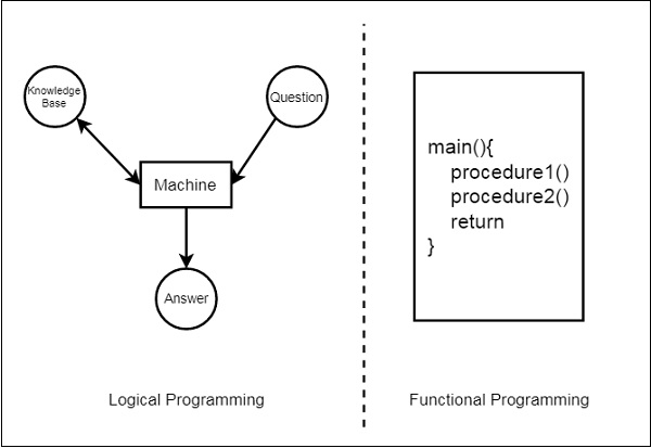
From this illustration, we can see that in Functional Programming, we have to define the procedures, and the rule how the procedures work. These procedures work step by step to solve one specific problem based on the algorithm. On the other hand, for the Logic Programming, we will provide knowledge base. Using this knowledge base, the machine can find answers to the given questions, which is totally different from functional programming.
In functional programming, we have to mention how one problem can be solved, but in logic programming we have to specify for which problem we actually want the solution. Then the logic programming automatically finds a suitable solution that will help us solve that specific problem.
Now let us see some more differences below −
| Functional Programming | Logic Programming |
|---|---|
| Functional Programming follows the Von-Neumann Architecture, or uses the sequential steps. | Logic Programming uses abstract model, or deals with objects and their relationships. |
| The syntax is actually the sequence of statements like (a, s, I). | The syntax is basically the logic formulae (Horn Clauses). |
| The computation takes part by executing the statements sequentially. | It computes by deducting the clauses. |
| Logic and controls are mixed together. | Logics and controls can be separated. |
What is Prolog?
Prolog or PROgramming in LOGics is a logical and declarative programming language. It is one major example of the fourth generation language that supports the declarative programming paradigm. This is particularly suitable for programs that involve symbolic or non-numeric computation. This is the main reason to use Prolog as the programming language in Artificial Intelligence, where symbol manipulation and inference manipulation are the fundamental tasks.
In Prolog, we need not mention the way how one problem can be solved, we just need to mention what the problem is, so that Prolog automatically solves it. However, in Prolog we are supposed to give clues as the solution method.
Prolog language basically has three different elements −
Facts − The fact is predicate that is true, for example, if we say, “Tom is the son of Jack”, then this is a fact.
Rules − Rules are extinctions of facts that contain conditional clauses. To satisfy a rule these conditions should be met. For example, if we define a rule as −
grandfather(X, Y) :- father(X, Z), parent(Z, Y)
This implies that for X to be the grandfather of Y, Z should be a parent of Y and X should be father of Z.
Questions − And to run a prolog program, we need some questions, and those questions can be answered by the given facts and rules.
History of Prolog
The heritage of prolog includes the research on theorem provers and some other automated deduction system that were developed in 1960s and 1970s. The Inference mechanism of the Prolog is based on Robinson’s Resolution Principle, that was proposed in 1965, and Answer extracting mechanism by Green (1968). These ideas came together forcefully with the advent of linear resolution procedures.
The explicit goal-directed linear resolution procedures, gave impetus to the development of a general purpose logic programming system. The first Prolog was the Marseille Prolog based on the work by Colmerauer in the year 1970. The manual of this Marseille Prolog interpreter (Roussel, 1975) was the first detailed description of the Prolog language.
Prolog is also considered as a fourth generation programming language supporting the declarative programming paradigm. The well-known Japanese Fifth-Generation Computer Project, that was announced in 1981, adopted Prolog as a development language, and thereby grabbed considerable attention on the language and its capabilities.
Some Applications of Prolog
Prolog is used in various domains. It plays a vital role in automation system. Following are some other important fields where Prolog is used −
-
Intelligent Database Retrieval
-
Natural Language Understanding
-
Specification Language
-
Machine Learning
-
Robot Planning
-
Automation System
-
Problem Solving
Prolog — Environment Setup
In this chapter, we will discuss how to install Prolog in our system.
Prolog Version
In this tutorial, we are using GNU Prolog, Version: 1.4.5
Official Website
This is the official GNU Prolog website where we can see all the necessary details about GNU Prolog, and also get the download link.
http://www.gprolog.org/
Direct Download Link
Given below are the direct download links of GNU Prolog for Windows. For other operating systems like Mac or Linux, you can get the download links by visiting the official website (Link is given above) −
http://www.gprolog.org/setup-gprolog-1.4.5-mingw-x86.exe (32 Bit System)
http://www.gprolog.org/setup-gprolog-1.4.5-mingw-x64.exe(64 Bit System)
Installation Guide
-
Download the exe file and run it.
-
You will see the window as shown below, then click on next −

Select proper directory where you want to install the software, otherwise let it be installed on the default directory. Then click on next.

You will get the below screen, simply go to next.

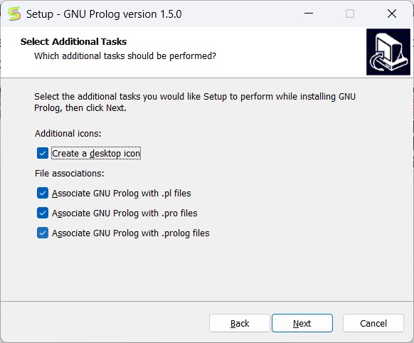
You can verify the below screen, and check/uncheck appropriate boxes, otherwise you can leave it as default. Then click on next.
In the next step, you will see the below screen, then click on Install.

Then wait for the installation process to finish.

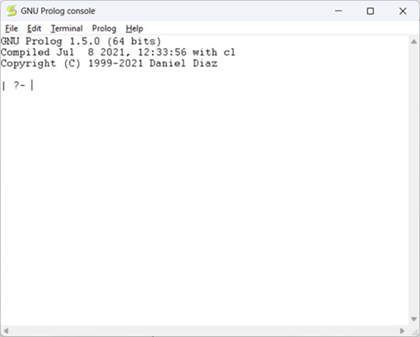
Finally click on Finish to start GNU Prolog.

The GNU prolog is installed successfully as shown below −
Prolog — Hello World
In the previous section, we have seen how to install GNU Prolog. Now, we will see how to write a simple Hello World program in our Prolog environment.
Hello World Program
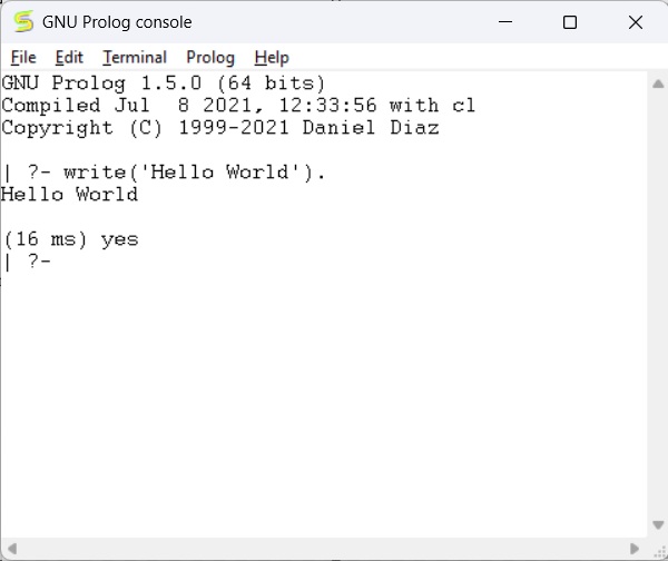
After running the GNU prolog, we can write hello world program directly from the console. To do so, we have to write the command as follows −
write('Hello World').
Note − After each line, you have to use one period (.) symbol to show that the line has ended.
The corresponding output will be as shown below −
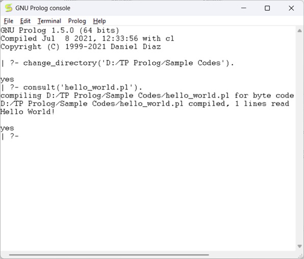
Now let us see how to run the Prolog script file (extension is *.pl) into the Prolog console.
Before running *.pl file, we must store the file into the directory where the GNU prolog console is pointing, otherwise just change the directory by the following steps −
Step 1 − From the prolog console, go to File > Change Dir, then click on that menu.
Step 2 − Select the proper folder and press OK.
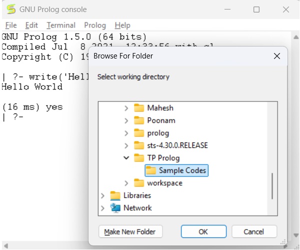
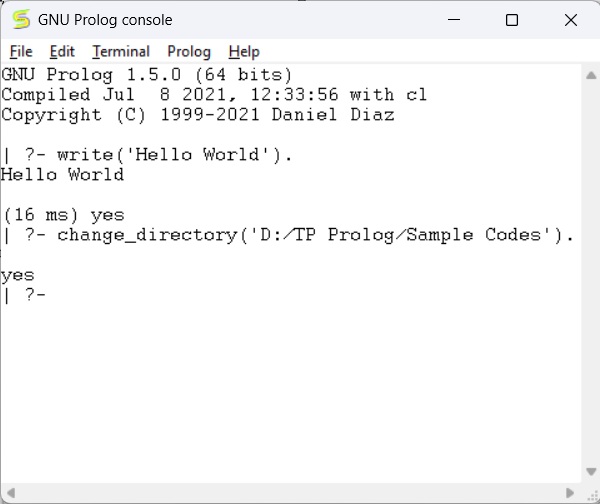
Now we can see in the prolog console, it shows that we have successfully changed the directory.
Step 3 − Now create one file (extension is *.pl) and write the code as follows −
main :- write('This is sample Prolog program'),
write(' This program is written into hello_world.pl file').
Now let’s run the code. To run it, we have to write the file name as follows −
[hello_world]
The output is as follows −
Prolog — Basics
In this chapter, we will gain some basic knowledge about Prolog. So we will move on to the first step of our Prolog Programming.
The different topics that will be covered in this chapter are −
Knowledge Base − This is one of the fundamental parts of Logic Programming. We will see in detail about the Knowledge Base, and how it helps in logic programming.
Facts, Rules and Queries − These are the building blocks of logic programming. We will get some detailed knowledge about facts and rules, and also see some kind of queries that will be used in logic programming.
Here, we will discuss about the essential building blocks of logic programming. These building blocks are Facts, Rules and the Queries.
Facts
We can define fact as an explicit relationship between objects, and properties these objects might have. So facts are unconditionally true in nature. Suppose we have some facts as given below −
-
Tom is a cat
-
Kunal loves to eat Pasta
-
Hair is black
-
Nawaz loves to play games
-
Pratyusha is lazy.
So these are some facts, that are unconditionally true. These are actually statements, that we have to consider as true.
Following are some guidelines to write facts −
-
Names of properties/relationships begin with lower case letters.
-
The relationship name appears as the first term.
-
Objects appear as comma-separated arguments within parentheses.
-
A period «.» must end a fact.
-
Objects also begin with lower case letters. They also can begin with digits (like 1234), and can be strings of characters enclosed in quotes e.g. color(penink, ‘red’).
-
phoneno(agnibha, 1122334455). is also called a predicate or clause.
Syntax
The syntax for facts is as follows −
relation(object1,object2...).
Example
Following is an example of the above concept −
cat(tom).
loves_to_eat(kunal,pasta).
of_color(hair,black).
loves_to_play_games(nawaz).
lazy(pratyusha).
Rules
We can define rule as an implicit relationship between objects. So facts are conditionally true. So when one associated condition is true, then the predicate is also true. Suppose we have some rules as given below −
-
Lili is happy if she dances.
-
Tom is hungry if he is searching for food.
-
Jack and Bili are friends if both of them love to play cricket.
-
will go to play if school is closed, and he is free.
So these are some rules that are conditionally true, so when the right hand side is true, then the left hand side is also true.
Here the symbol ( :- ) will be pronounced as “If”, or “is implied by”. This is also known as neck symbol, the LHS of this symbol is called the Head, and right hand side is called Body. Here we can use comma (,) which is known as conjunction, and we can also use semicolon, that is known as disjunction.
Syntax
rule_name(object1, object2, ...) :- fact/rule(object1,
 object2, ...)
Suppose a clause is like :
P :- Q;R.
This can also be written as
P :- Q.
P :- R.

If one clause is like :
P :- Q,R;S,T,U.

Is understood as
P :- (Q,R);(S,T,U).
Or can also be written as:
P :- Q,R.
P :- S,T,U.
Example
happy(lili) :- dances(lili).
hungry(tom) :- search_for_food(tom).
friends(jack, bili) :- lovesCricket(jack), lovesCricket(bili).
goToPlay(ryan) :- isClosed(school), free(ryan).
Queries
Queries are some questions on the relationships between objects and object properties. So question can be anything, as given below −
-
Is tom a cat?
-
Does Kunal love to eat pasta?
-
Is Lili happy?
-
Will Ryan go to play?
So according to these queries, Logic programming language can find the answer and return them.
Knowledge Base in Logic Programming
In this section, we will see what knowledge base in logic programming is.
Well, as we know there are three main components in logic programming − Facts, Rules and Queries. Among these three if we collect the facts and rules as a whole then that forms a Knowledge Base. So we can say that the knowledge base is a collection of facts and rules.
Now, we will see how to write some knowledge bases. Suppose we have our very first knowledge base called KB1. Here in the KB1, we have some facts. The facts are used to state things, that are unconditionally true of the domain of interest.
Knowledge Base 1
Suppose we have some knowledge, that Priya, Tiyasha, and Jaya are three girls, among them, Priya can cook. Let’s try to write these facts in a more generic way as shown below −
girl(priya).
girl(tiyasha).
girl(jaya).
can_cook(priya).
Note − Here we have written the name in lowercase letters, because in Prolog, a string starting with uppercase letter indicates a variable.
Now we can use this knowledge base by posing some queries. “Is priya a girl?”, it will reply “yes”, “is jamini a girl?” then it will answer “No”, because it does not know who jamini is. Our next question is “Can Priya cook?”, it will say “yes”, but if we ask the same question for Jaya, it will say “No”.
Output
GNU Prolog 1.4.5 (64 bits)
Compiled Jul 14 2018, 13:19:42 with x86_64-w64-mingw32-gcc
By Daniel Diaz
Copyright (C) 1999-2018 Daniel Diaz
| ?- change_directory('D:/TP Prolog/Sample_Codes').

yes
| ?- [kb1]
.
compiling D:/TP Prolog/Sample_Codes/kb1.pl for byte code...
D:/TP Prolog/Sample_Codes/kb1.pl compiled, 3 lines read - 489 bytes written, 10 ms

yes
| ?- girl(priya)
.

yes
| ?- girl(jamini).

no
| ?- can_cook(priya).

yes
| ?- can_cook(jaya).

no
| ?-
Let us see another knowledge base, where we have some rules. Rules contain some information that are conditionally true about the domain of interest. Suppose our knowledge base is as follows −
sing_a_song(ananya).
listens_to_music(rohit).

listens_to_music(ananya) :- sing_a_song(ananya).
happy(ananya) :- sing_a_song(ananya).
happy(rohit) :- listens_to_music(rohit).
playes_guitar(rohit) :- listens_to_music(rohit).
So there are some facts and rules given above. The first two are facts, but the rest are rules. As we know that Ananya sings a song, this implies she also listens to music. So if we ask “Does Ananya listen to music?”, the answer will be true. Similarly, “is Rohit happy?”, this will also be true because he listens to music. But if our question is “does Ananya play guitar?”, then according to the knowledge base, it will say “No”. So these are some examples of queries based on this Knowledge base.
Output
| ?- [kb2].
compiling D:/TP Prolog/Sample_Codes/kb2.pl for byte code...
D:/TP Prolog/Sample_Codes/kb2.pl compiled, 6 lines read - 1066 bytes written, 15 ms

yes
| ?- happy(rohit).

yes
| ?- sing_a_song(rohit).

no
| ?- sing_a_song(ananya).

yes
| ?- playes_guitar(rohit).

yes
| ?- playes_guitar(ananya).

no
| ?- listens_to_music(ananya).

yes
| ?-
Knowledge Base 3
The facts and rules of Knowledge Base 3 are as follows −
can_cook(priya).
can_cook(jaya).
can_cook(tiyasha).

likes(priya,jaya) :- can_cook(jaya).
likes(priya,tiyasha) :- can_cook(tiyasha).
Suppose we want to see the members who can cook, we can use one variable in our query. The variables should start with uppercase letters. In the result, it will show one by one. If we press enter, then it will come out, otherwise if we press semicolon (;), then it will show the next result.
Let us see one practical demonstration output to understand how it works.
Output
| ?- [kb3].
compiling D:/TP Prolog/Sample_Codes/kb3.pl for byte code...
D:/TP Prolog/Sample_Codes/kb3.pl compiled, 5 lines read - 737 bytes written, 22 ms
warning: D:/TP Prolog/Sample_Codes/kb3.pl:1: redefining procedure can_cook/1
         D:/TP Prolog/Sample_Codes/kb1.pl:4: previous definition

yes
| ?- can_cook(X).

X = priya ? ;

X = jaya ? ;

X = tiyasha

yes
| ?- likes(priya,X).

X = jaya ? ;

X = tiyasha

yes
| ?-
Prolog — Relations
Relationship is one of the main features that we have to properly mention in Prolog. These relationships can be expressed as facts and rules. After that we will see about the family relationships, how we can express family based relationships in Prolog, and also see the recursive relationships of the family.
We will create the knowledge base by creating facts and rules, and play query on them.
Relations in Prolog
In Prolog programs, it specifies relationship between objects and properties of the objects.
Suppose, there’s a statement, “Amit has a bike”, then we are actually declaring the ownership relationship between two objects — one is Amit and the other is bike.
If we ask a question, “Does Amit own a bike?”, we are actually trying to find out about one relationship.
There are various kinds of relationships, of which some can be rules as well. A rule can find out about a relationship even if the relationship is not defined explicitly as a fact.
We can define a brother relationship as follows −
Two person are brothers, if,
-
They both are male.
-
They have the same parent.
Now consider we have the below phrases −
-
parent(sudip, piyus).
-
parent(sudip, raj).
-
male(piyus).
-
male(raj).
-
brother(X,Y) :- parent(Z,X), parent(Z,Y),male(X), male(Y)
These clauses can give us the answer that piyus and raj are brothers, but we will get three pairs of output here. They are: (piyus, piyus), (piyus, raj), (raj, raj). For these pairs, given conditions are true, but for the pairs (piyus, piyus), (raj, raj), they are not actually brothers, they are the same persons. So we have to create the clauses properly to form a relationship.
The revised relationship can be as follows −
A and B are brothers if −
-
A and B, both are male
-
They have same father
-
They have same mother
-
A and B are not same
Family Relationship in Prolog
Here we will see the family relationship. This is an example of complex relationship that can be formed using Prolog. We want to make a family tree, and that will be mapped into facts and rules, then we can run some queries on them.
Suppose the family tree is as follows −
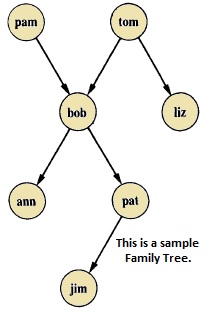
Here from this tree, we can understand that there are few relationships. Here bob is a child of pam and tom, and bob also has two children — ann and pat. Bob has one brother liz, whose parent is also tom. So we want to make predicates as follows −
Predicates
-
parent(pam, bob).
-
parent(tom, bob).
-
parent(tom, liz).
-
parent(bob, ann).
-
parent(bob, pat).
-
parent(pat, jim).
-
parent(bob, peter).
-
parent(peter, jim).
From our example, it has helped to illustrate some important points −
-
We have defined parent relation by stating the n-tuples of objects based on the given info in the family tree.
-
The user can easily query the Prolog system about relations defined in the program.
-
A Prolog program consists of clauses terminated by a full stop.
-
The arguments of relations can (among other things) be: concrete objects, or constants (such as pat and jim), or general objects such as X and Y. Objects of the first kind in our program are called atoms. Objects of the second kind are called variables.
-
Questions to the system consist of one or more goals.
Some facts can be written in two different ways, like sex of family members can be written in either of the forms −
-
female(pam).
-
male(tom).
-
male(bob).
-
female(liz).
-
female(pat).
-
female(ann).
-
male(jim).
Or in the below form −
-
sex( pam, feminine).
-
sex( tom, masculine).
-
sex( bob, masculine).
-
… and so on.
Now if we want to make mother and sister relationship, then we can write as given below −
In Prolog syntax, we can write −
-
mother(X,Y) :- parent(X,Y), female(X).
-
sister(X,Y) :- parent(Z,X), parent(Z,Y), female(X), X == Y.
Now let us see the practical demonstration −
Knowledge Base (family.pl)
female(pam).
female(liz).
female(pat).
female(ann).
male(jim).
male(bob).
male(tom).
male(peter).
parent(pam,bob).
parent(tom,bob).
parent(tom,liz).
parent(bob,ann).
parent(bob,pat).
parent(pat,jim).
parent(bob,peter).
parent(peter,jim).
mother(X,Y):- parent(X,Y),female(X).
father(X,Y):- parent(X,Y),male(X).
haschild(X):- parent(X,_).
sister(X,Y):- parent(Z,X),parent(Z,Y),female(X),X==Y.
brother(X,Y):-parent(Z,X),parent(Z,Y),male(X),X==Y.
Output
| ?- [family].
compiling D:/TP Prolog/Sample_Codes/family.pl for byte code...
D:/TP Prolog/Sample_Codes/family.pl compiled, 23 lines read - 3088 bytes written, 9 ms

yes
| ?- parent(X,jim).

X = pat ? ;

X = peter

yes
| ?-
mother(X,Y).

X = pam
Y = bob ? ;

X = pat
Y = jim ? ;

no
| ?- haschild(X).

X = pam ? ;

X = tom ? ;

X = tom ? ;

X = bob ? ;

X = bob ? ;

X = pat ? ;

X = bob ? ;

X = peter

yes
| ?- sister(X,Y).

X = liz
Y = bob ? ;

X = ann
Y = pat ? ;

X = ann
Y = peter ? ;

X = pat
Y = ann ? ;

X = pat
Y = peter ? ;

(16 ms) no
| ?-
Now let us see some more relationships that we can make from the previous relationships of a family. So if we want to make a grandparent relationship, that can be formed as follows −
We can also create some other relationships like wife, uncle, etc. We can write the relationships as given below −
-
grandparent(X,Y) :- parent(X,Z), parent(Z,Y).
-
grandmother(X,Z) :- mother(X,Y), parent(Y,Z).
-
grandfather(X,Z) :- father(X,Y), parent(Y,Z).
-
wife(X,Y) :- parent(X,Z),parent(Y,Z), female(X),male(Y).
-
uncle(X,Z) :- brother(X,Y), parent(Y,Z).
So let us write a prolog program to see this in action. Here we will also see the trace to trace-out the execution.
Knowledge Base (family_ext.pl)
female(pam).
female(liz).
female(pat).
female(ann).

male(jim).
male(bob).
male(tom).
male(peter).

parent(pam,bob).
parent(tom,bob).
parent(tom,liz).
parent(bob,ann).

parent(bob,pat).
parent(pat,jim).
parent(bob,peter).
parent(peter,jim).

mother(X,Y):- parent(X,Y),female(X).
father(X,Y):-parent(X,Y),male(X).
sister(X,Y):-parent(Z,X),parent(Z,Y),female(X),X==Y.
brother(X,Y):-parent(Z,X),parent(Z,Y),male(X),X==Y.
grandparent(X,Y):-parent(X,Z),parent(Z,Y).
grandmother(X,Z):-mother(X,Y),parent(Y,Z).
grandfather(X,Z):-father(X,Y),parent(Y,Z).
wife(X,Y):-parent(X,Z),parent(Y,Z),female(X),male(Y).
uncle(X,Z):-brother(X,Y),parent(Y,Z).
Output
| ?- [family_ext].
compiling D:/TP Prolog/Sample_Codes/family_ext.pl for byte code...
D:/TP Prolog/Sample_Codes/family_ext.pl compiled, 27 lines read - 4646 bytes written, 10 ms

| ?- uncle(X,Y).

X = peter
Y = jim ? ;

no
| ?- grandparent(X,Y).

X = pam
Y = ann ? ;

X = pam
Y = pat ? ;

X = pam
Y = peter ? ;

X = tom
Y = ann ? ;

X = tom
Y = pat ? ;

X = tom
Y = peter ? ;

X = bob
Y = jim ? ;

X = bob
Y = jim ? ;

no
| ?- wife(X,Y).

X = pam
Y = tom ? ;

X = pat
Y = peter ? ;

(15 ms) no
| ?-
Tracing the output
In Prolog we can trace the execution. To trace the output, you have to enter into the trace mode by typing “trace.”. Then from the output we can see that we are just tracing “pam is mother of whom?”. See the tracing output by taking X = pam, and Y as variable, there Y will be bob as answer. To come out from the tracing mode press “notrace.”
Program
| ?- [family_ext].
compiling D:/TP Prolog/Sample_Codes/family_ext.pl for byte code...
D:/TP Prolog/Sample_Codes/family_ext.pl compiled, 27 lines read - 4646 bytes written, 10 ms

(16 ms) yes
| ?- mother(X,Y).

X = pam
Y = bob ? ;

X = pat
Y = jim ? ;

no
| ?- trace.
The debugger will first creep -- showing everything (trace)

yes
{trace}
| ?- mother(pam,Y).
   1 1 Call: mother(pam,_23) ?
   2 2 Call: parent(pam,_23) ?
   2 2 Exit: parent(pam,bob) ?
   3 2 Call: female(pam) ?
   3 2 Exit: female(pam) ?
   1 1 Exit: mother(pam,bob) ?

Y = bob

(16 ms) yes
{trace}
| ?- notrace.
The debugger is switched off

yes
| ?-
Recursion in Family Relationship
In the previous section, we have seen that we can define some family relationships. These relationships are static in nature. We can also create some recursive relationships which can be expressed from the following illustration −
So we can understand that predecessor relationship is recursive. We can express this relationship using the following syntax −
predecessor(X, Z) :- parent(X, Z).
predecessor(X, Z) :- parent(X, Y),predecessor(Y, Z).
Now let us see the practical demonstration.
Knowledge Base (family_rec.pl)
female(pam).
female(liz).
female(pat).
female(ann).

male(jim).
male(bob).
male(tom).
male(peter).

parent(pam,bob).
parent(tom,bob).
parent(tom,liz).
parent(bob,ann).
parent(bob,pat).
parent(pat,jim).
parent(bob,peter).
parent(peter,jim).

predecessor(X, Z) :- parent(X, Z).
predecessor(X, Z) :- parent(X, Y),predecessor(Y, Z).
Output
| ?- [family_rec].
compiling D:/TP Prolog/Sample_Codes/family_rec.pl for byte code...
D:/TP Prolog/Sample_Codes/family_rec.pl compiled, 21 lines read - 1851 bytes written, 14 ms

yes
| ?- predecessor(peter,X).

X = jim ? ;

no
| ?- trace.
The debugger will first creep -- showing everything (trace)

yes
{trace}
| ?- predecessor(bob,X).
   1 1 Call: predecessor(bob,_23) ?
   2 2 Call: parent(bob,_23) ?
   2 2 Exit: parent(bob,ann) ?
   1 1 Exit: predecessor(bob,ann) ?

X = ann ? ;
   1 1 Redo: predecessor(bob,ann) ?
   2 2 Redo: parent(bob,ann) ?
   2 2 Exit: parent(bob,pat) ?
   1 1 Exit: predecessor(bob,pat) ?

X = pat ? ;
   1 1 Redo: predecessor(bob,pat) ?
   2 2 Redo: parent(bob,pat) ?
   2 2 Exit: parent(bob,peter) ?
   1 1 Exit: predecessor(bob,peter) ?

X = peter ? ;
   1 1 Redo: predecessor(bob,peter) ?
   2 2 Call: parent(bob,_92) ?
   2 2 Exit: parent(bob,ann) ?
   3 2 Call: predecessor(ann,_23) ?
   4 3 Call: parent(ann,_23) ?
   4 3 Fail: parent(ann,_23) ?
   4 3 Call: parent(ann,_141) ?
   4 3 Fail: parent(ann,_129) ?
   3 2 Fail: predecessor(ann,_23) ?
   2 2 Redo: parent(bob,ann) ?
   2 2 Exit: parent(bob,pat) ?
   3 2 Call: predecessor(pat,_23) ?
   4 3 Call: parent(pat,_23) ?
   4 3 Exit: parent(pat,jim) ?
   3 2 Exit: predecessor(pat,jim) ?
   1 1 Exit: predecessor(bob,jim) ?

X = jim ? ;
   1 1 Redo: predecessor(bob,jim) ?
   3 2 Redo: predecessor(pat,jim) ?
   4 3 Call: parent(pat,_141) ?
   4 3 Exit: parent(pat,jim) ?
   5 3 Call: predecessor(jim,_23) ?
   6 4 Call: parent(jim,_23) ?
   6 4 Fail: parent(jim,_23) ?
   6 4 Call: parent(jim,_190) ?
   6 4 Fail: parent(jim,_178) ?
   5 3 Fail: predecessor(jim,_23) ?
   3 2 Fail: predecessor(pat,_23) ?
   2 2 Redo: parent(bob,pat) ?
   2 2 Exit: parent(bob,peter) ?
   3 2 Call: predecessor(peter,_23) ?
   4 3 Call: parent(peter,_23) ?
   4 3 Exit: parent(peter,jim) ?
   3 2 Exit: predecessor(peter,jim) ?
   1 1 Exit: predecessor(bob,jim) ?

X = jim ?

(78 ms) yes
{trace}
| ?-
Prolog — Data Objects
In this chapter, we will learn data objects in Prolog. They can be divided into few different categories as shown below −
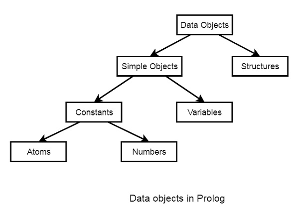
Below are some examples of different kinds of data objects −
-
Atoms − tom, pat, x100, x_45
-
Numbers − 100, 1235, 2000.45
-
Variables − X, Y, Xval, _X
-
Structures − day(9, jun, 2017), point(10, 25)
Atoms and Variables
In this section, we will discuss the atoms, numbers and the variables of Prolog.
Atoms
Atoms are one variation of constants. They can be any names or objects. There are few rules that should be followed when we are trying to use Atoms as given below −
Strings of letters, digits and the underscore character, ‘_’, starting with a lower-case letter. For example −
-
azahar
-
b59
-
b_59
-
b_59AB
-
b_x25
-
antara_sarkar
Strings of special characters
We have to keep in mind that when using atoms of this form, some care is necessary as some strings of special characters already have a predefined meaning; for example ‘:-‘.
-
<—>
-
=======>
-
…
-
.:.
-
::=
Strings of characters enclosed in single quotes.
This is useful if we want to have an atom that starts with a capital letter. By enclosing it in quotes, we make it distinguishable from variables −
-
‘Rubai’
-
‘Arindam_Chatterjee’
-
‘Sumit Mitra’
Numbers
Another variation of constants is the Numbers. So integer numbers can be represented as 100, 4, -81, 1202. In Prolog, the normal range of integers is from -16383 to 16383.
Prolog also supports real numbers, but normally the use-case of floating point number is very less in Prolog programs, because Prolog is for symbolic, non-numeric computation. The treatment of real numbers depends on the implementation of Prolog. Example of real numbers are 3.14159, -0.00062, 450.18, etc.
The variables come under the Simple Objects section. Variables can be used in many such cases in our Prolog program, that we have seen earlier. So there are some rules of defining variables in Prolog.
We can define Prolog variables, such that variables are strings of letters, digits and underscore characters. They start with an upper-case letter or an underscore character. Some examples of Variables are −
-
X
-
Sum
-
Memer_name
-
Student_list
-
Shoppinglist
-
_a50
-
_15
Anonymous Variables in Prolog
Anonymous variables have no names. The anonymous variables in prolog is written by a single underscore character ‘_’. And one important thing is that each individual anonymous variable is treated as different. They are not same.
Now the question is, where should we use these anonymous variables?
Suppose in our knowledge base we have some facts — “jim hates tom”, “pat hates bob”. So if tom wants to find out who hates him, then he can use variables. However, if he wants to check whether there is someone who hates him, we can use anonymous variables. So when we want to use the variable, but do not want to reveal the value of the variable, then we can use anonymous variables.
So let us see its practical implementation −
Knowledge Base (var_anonymous.pl)
hates(jim,tom).
hates(pat,bob).
hates(dog,fox).
hates(peter,tom).
Output
| ?- [var_anonymous].
compiling D:/TP Prolog/Sample_Codes/var_anonymous.pl for byte code...
D:/TP Prolog/Sample_Codes/var_anonymous.pl compiled, 3 lines read - 536 bytes written, 16 ms

yes
| ?- hates(X,tom).

X = jim ? ;

X = peter

yes
| ?- hates(_,tom).

true ? ;

(16 ms) yes
| ?- hates(_,pat).

no
| ?- hates(_,fox).

true ? ;

no
| ?-
Prolog — Operators
In the following sections, we will see what are the different types of operators in Prolog. Types of the comparison operators and Arithmetic operators.
We will also see how these are different from any other high level language operators, how they are syntactically different, and how they are different in their work. Also we will see some practical demonstration to understand the usage of different operators.
Comparison Operators
Comparison operators are used to compare two equations or states. Following are different comparison operators −
| Operator | Meaning |
|---|---|
| X > Y | X is greater than Y |
| X < Y | X is less than Y |
| X >= Y | X is greater than or equal to Y |
| X =< Y | X is less than or equal to Y |
| X =:= Y | the X and Y values are equal |
| X == Y | the X and Y values are not equal |
You can see that the ‘=<’ operator, ‘=:=’ operator and ‘==’ operators are syntactically different from other languages. Let us see some practical demonstration to this.
Example
| ?- 1+2=:=2+1.

yes
| ?- 1+2=2+1.

no
| ?- 1+A=B+2.

A = 2
B = 1

yes
| ?- 5<10.

yes
| ?- 5>10.

no
| ?- 10==100.

yes
Here we can see 1+2=:=2+1 is returning true, but 1+2=2+1 is returning false. This is because, in the first case it is checking whether the value of 1 + 2 is same as 2 + 1 or not, and the other one is checking whether two patterns ‘1+2’ and ‘2+1’ are same or not. As they are not same, it returns no (false). In the case of 1+A=B+2, A and B are two variables, and they are automatically assigned to some values that will match the pattern.
Arithmetic Operators in Prolog
Arithmetic operators are used to perform arithmetic operations. There are few different types of arithmetic operators as follows −
| Operator | Meaning |
|---|---|
| + | Addition |
| — | Subtraction |
| * | Multiplication |
| / | Division |
| ** | Power |
| // | Integer Division |
| mod | Modulus |
Let us see one practical code to understand the usage of these operators.
Program
calc :- X is 100 + 200,write('100 + 200 is '),write(X),nl,
        Y is 400 - 150,write('400 - 150 is '),write(Y),nl,
        Z is 10 * 300,write('10 * 300 is '),write(Z),nl,
        A is 100 / 30,write('100 / 30 is '),write(A),nl,
        B is 100 // 30,write('100 // 30 is '),write(B),nl,
        C is 100 ** 2,write('100 ** 2 is '),write(C),nl,
        D is 100 mod 30,write('100 mod 30 is '),write(D),nl.
Note − The nl is used to create new line.
Output
| ?- change_directory('D:/TP Prolog/Sample_Codes').

yes
| ?- [op_arith].
compiling D:/TP Prolog/Sample_Codes/op_arith.pl for byte code...
D:/TP Prolog/Sample_Codes/op_arith.pl compiled, 6 lines read - 2390 bytes written, 11 ms

yes
| ?- calc.
100 + 200 is 300
400 - 150 is 250
10 * 300 is 3000
100 / 30 is 3.3333333333333335
100 // 30 is 3
100 ** 2 is 10000.0
100 mod 30 is 10

yes
| ?-
Prolog — Loop & Decision Making
In this chapter, we will discuss loops and decision making in Prolog.
Loops
Loop statements are used to execute the code block multiple times. In general, for, while, do-while are loop constructs in programming languages (like Java, C, C++).
Code block is executed multiple times using recursive predicate logic. There are no direct loops in some other languages, but we can simulate loops with few different techniques.
Program
count_to_10(10) :- write(10),nl.
count_to_10(X) :-
   write(X),nl,
   Y is X + 1,
   count_to_10(Y).
Output
| ?- [loop].
compiling D:/TP Prolog/Sample_Codes/loop.pl for byte code...
D:/TP Prolog/Sample_Codes/loop.pl compiled, 4 lines read - 751 bytes written, 16 ms

(16 ms) yes
| ?- count_to_10(3).
3
4
5
6
7
8
9
10

true ?
yes
| ?-
Now create a loop that takes lowest and highest values. So, we can use the between() to simulate loops.
Program
Let us see an example program −
count_down(L, H) :-
   between(L, H, Y),
   Z is H - Y,
   write(Z), nl.

count_up(L, H) :-
   between(L, H, Y),
   Z is L + Y,
   write(Z), nl.
Output
| ?- [loop].
compiling D:/TP Prolog/Sample_Codes/loop.pl for byte code...
D:/TP Prolog/Sample_Codes/loop.pl compiled, 14 lines read - 1700 bytes written, 16 ms

yes
| ?- count_down(12,17).
5

true ? ;
4

true ? ;
3

true ? ;
2

true ? ;
1

true ? ;
0

yes
| ?- count_up(5,12).
10

true ? ;
11

true ? ;
12

true ? ;
13

true ? ;
14

true ? ;
15

true ? ;
16

true ? ;
17

yes
| ?-
Decision Making
The decision statements are If-Then-Else statements. So when we try to match some condition, and perform some task, then we use the decision making statements. The basic usage is as follows −
If <condition> is true, Then <do this>, Else
In some different programming languages, there are If-Else statements, but in Prolog we have to define our statements in some other manner. Following is an example of decision making in Prolog.
Program
% If-Then-Else statement

gt(X,Y) :- X >= Y,write('X is greater or equal').
gt(X,Y) :- X < Y,write('X is smaller').

% If-Elif-Else statement

gte(X,Y) :- X > Y,write('X is greater').
gte(X,Y) :- X =:= Y,write('X and Y are same').
gte(X,Y) :- X < Y,write('X is smaller').
Output
| ?- [test].
compiling D:/TP Prolog/Sample_Codes/test.pl for byte code...
D:/TP Prolog/Sample_Codes/test.pl compiled, 3 lines read - 529 bytes written, 15 ms

yes
| ?- gt(10,100).
X is smaller

yes
| ?- gt(150,100).
X is greater or equal

true ?

yes
| ?- gte(10,20).
X is smaller

(15 ms) yes
| ?- gte(100,20).
X is greater

true ?

yes
| ?- gte(100,100).
X and Y are same

true ?

yes
| ?-
Prolog — Conjunctions & Disjunctions
In this chapter, we shall discuss Conjunction and Disjunction properties. These properties are used in other programming languages using AND and OR logics. Prolog also uses the same logic in its syntax.
Conjunction
Conjunction (AND logic) can be implemented using the comma (,) operator. So two predicates separated by comma are joined with AND statement. Suppose we have a predicate, parent(jhon, bob), which means “Jhon is parent of Bob”, and another predicate, male(jhon), which means “Jhon is male”. So we can make another predicate that father(jhon,bob), which means “Jhon is father of Bob”. We can define predicate father, when he is parent AND he is male.
Disjunction
Disjunction (OR logic) can be implemented using the semi-colon (;) operator. So two predicates separated by semi-colon are joined with OR statement. Suppose we have a predicate, father(jhon, bob). This tells that “Jhon is father of Bob”, and another predicate, mother(lili,bob), this tells that “lili is mother of bob”. If we create another predicate as child(), this will be true when father(jhon, bob) is true OR mother(lili,bob) is true.
Program
parent(jhon,bob).
parent(lili,bob).

male(jhon).
female(lili).

% Conjunction Logic
father(X,Y) :- parent(X,Y),male(X).
mother(X,Y) :- parent(X,Y),female(X).

% Disjunction Logic
child_of(X,Y) :- father(X,Y);mother(X,Y).
Output
| ?- [conj_disj].
compiling D:/TP Prolog/Sample_Codes/conj_disj.pl for byte code...
D:/TP Prolog/Sample_Codes/conj_disj.pl compiled, 11 lines read - 1513 bytes written, 24 ms

yes
| ?- father(jhon,bob).

yes
| ?- child_of(jhon,bob).

true ?

yes
| ?- child_of(lili,bob).

yes
| ?-
Prolog — Lists
In this chapter, we will discuss one of the important concepts in Prolog, The Lists. It is a data structure that can be used in different cases for non-numeric programming. Lists are used to store the atoms as a collection.
In the subsequent sections, we will discuss the following topics −
-
Representation of lists in Prolog
-
Basic operations on prolog such as Insert, delete, update, append.
-
Repositioning operators such as permutation, combination, etc.
-
Set operations like set union, set intersection, etc.
Representation of Lists
The list is a simple data structure that is widely used in non-numeric programming. List consists of any number of items, for example, red, green, blue, white, dark. It will be represented as, [red, green, blue, white, dark]. The list of elements will be enclosed with square brackets.
A list can be either empty or non-empty. In the first case, the list is simply written as a Prolog atom, []. In the second case, the list consists of two things as given below −
-
The first item, called the head of the list;
-
The remaining part of the list, called the tail.
Suppose we have a list like: [red, green, blue, white, dark]. Here the head is red and tail is [green, blue, white, dark]. So the tail is another list.
Now, let us consider we have a list, L = [a, b, c]. If we write Tail = [b, c] then we can also write the list L as L = [ a | Tail]. Here the vertical bar (|) separates the head and tail parts.
So the following list representations are also valid −
-
[a, b, c] = [x | [b, c] ]
-
[a, b, c] = [a, b | [c] ]
-
[a, b, c] = [a, b, c | [ ] ]
For these properties we can define the list as −
A data structure that is either empty or consists of two parts − a head and a tail. The tail itself has to be a list.
Basic Operations on Lists
Following table contains various operations on prolog lists −
| Operations | Definition |
|---|---|
| Membership Checking | During this operation, we can verify whether a given element is member of specified list or not? |
| Length Calculation | With this operation, we can find the length of a list. |
| Concatenation | Concatenation is an operation which is used to join/add two lists. |
| Delete Items | This operation removes the specified element from a list. |
| Append Items | Append operation adds one list into another (as an item). |
| Insert Items | This operation inserts a given item into a list. |
Membership Operation
During this operation, we can check whether a member X is present in list L or not? So how to check this? Well, we have to define one predicate to do so. Suppose the predicate name is list_member(X,L). The goal of this predicate is to check whether X is present in L or not.
To design this predicate, we can follow these observations. X is a member of L if either −
-
X is head of L, or
-
X is a member of the tail of L
Program
list_member(X,[X|_]).
list_member(X,[_|TAIL]) :- list_member(X,TAIL).
Output
| ?- [list_basics].
compiling D:/TP Prolog/Sample_Codes/list_basics.pl for byte code...
D:/TP Prolog/Sample_Codes/list_basics.pl compiled, 1 lines read - 467 bytes written, 13 ms

yes
| ?- list_member(b,[a,b,c]).

true ?

yes
| ?- list_member(b,[a,[b,c]]).

no
| ?- list_member([b,c],[a,[b,c]]).

true ?

yes
| ?- list_member(d,[a,b,c]).

no
| ?- list_member(d,[a,b,c]).
Length Calculation
This is used to find the length of list L. We will define one predicate to do this task. Suppose the predicate name is list_length(L,N). This takes L and N as input argument. This will count the elements in a list L and instantiate N to their number. As was the case with our previous relations involving lists, it is useful to consider two cases −
-
If list is empty, then length is 0.
-
If the list is not empty, then L = [Head|Tail], then its length is 1 + length of Tail.
Program
list_length([],0).
list_length([_|TAIL],N) :- list_length(TAIL,N1), N is N1 + 1.
Output
| ?- [list_basics].
compiling D:/TP Prolog/Sample_Codes/list_basics.pl for byte code...
D:/TP Prolog/Sample_Codes/list_basics.pl compiled, 4 lines read - 985 bytes written, 23 ms

yes
| ?- list_length([a,b,c,d,e,f,g,h,i,j],Len).

Len = 10

yes
| ?- list_length([],Len).

Len = 0

yes
| ?- list_length([[a,b],[c,d],[e,f]],Len).

Len = 3

yes
| ?-
Concatenation
Concatenation of two lists means adding the list items of the second list after the first one. So if two lists are [a,b,c] and [1,2], then the final list will be [a,b,c,1,2]. So to do this task we will create one predicate called list_concat(), that will take first list L1, second list L2, and the L3 as resultant list. There are two observations here.
-
If the first list is empty, and second list is L, then the resultant list will be L.
-
If the first list is not empty, then write this as [Head|Tail], concatenate Tail with L2 recursively, and store into new list in the form, [Head|New List].
Program
list_concat([],L,L).
list_concat([X1|L1],L2,[X1|L3]) :- list_concat(L1,L2,L3).
Output
| ?- [list_basics].
compiling D:/TP Prolog/Sample_Codes/list_basics.pl for byte code...
D:/TP Prolog/Sample_Codes/list_basics.pl compiled, 7 lines read - 1367 bytes written, 19 ms

yes
| ?- list_concat([1,2],[a,b,c],NewList).

NewList = [1,2,a,b,c]

yes
| ?- list_concat([],[a,b,c],NewList).

NewList = [a,b,c]

yes
| ?- list_concat([[1,2,3],[p,q,r]],[a,b,c],NewList).

NewList = [[1,2,3],[p,q,r],a,b,c]

yes
| ?-
Delete from List
Suppose we have a list L and an element X, we have to delete X from L. So there are three cases −
-
If X is the only element, then after deleting it, it will return empty list.
-
If X is head of L, the resultant list will be the Tail part.
-
If X is present in the Tail part, then delete from there recursively.
Program
list_delete(X, [X], []).
list_delete(X,[X|L1], L1).
list_delete(X, [Y|L2], [Y|L1]) :- list_delete(X,L2,L1).
Output
| ?- [list_basics].
compiling D:/TP Prolog/Sample_Codes/list_basics.pl for byte code...
D:/TP Prolog/Sample_Codes/list_basics.pl compiled, 11 lines read - 1923 bytes written, 25 ms

yes
| ?- list_delete(a,[a,e,i,o,u],NewList).

NewList = [e,i,o,u] ?

yes
| ?- list_delete(a,[a],NewList).

NewList = [] ?

yes
| ?- list_delete(X,[a,e,i,o,u],[a,e,o,u]).

X = i ? ;

no
| ?-
Append into List
Appending two lists means adding two lists together, or adding one list as an item. Now if the item is present in the list, then the append function will not work. So we will create one predicate namely, list_append(L1, L2, L3). The following are some observations −
-
Let A is an element, L1 is a list, the output will be L1 also, when L1 has A already.
-
Otherwise new list will be L2 = [A|L1].
Program
list_member(X,[X|_]).
list_member(X,[_|TAIL]) :- list_member(X,TAIL).

list_append(A,T,T) :- list_member(A,T),!.
list_append(A,T,[A|T]).
In this case, we have used (!) symbol, that is known as cut. So when the first line is executed successfully, then we cut it, so it will not execute the next operation.
Output
| ?- [list_basics].
compiling D:/TP Prolog/Sample_Codes/list_basics.pl for byte code...
D:/TP Prolog/Sample_Codes/list_basics.pl compiled, 14 lines read - 2334 bytes written, 25 ms

(16 ms) yes
| ?- list_append(a,[e,i,o,u],NewList).

NewList = [a,e,i,o,u]

yes
| ?- list_append(e,[e,i,o,u],NewList).

NewList = [e,i,o,u]

yes
| ?- list_append([a,b],[e,i,o,u],NewList).

NewList = [[a,b],e,i,o,u]

yes
| ?-
Insert into List
This method is used to insert an item X into list L, and the resultant list will be R. So the predicate will be in this form list_insert(X, L, R). So this can insert X into L in all possible positions. If we see closer, then there are some observations.
-
If we perform list_insert(X,L,R), we can use list_delete(X,R,L), so delete X from R and make new list L.
Program
list_delete(X, [X], []).
list_delete(X,[X|L1], L1).
list_delete(X, [Y|L2], [Y|L1]) :- list_delete(X,L2,L1).

list_insert(X,L,R) :- list_delete(X,R,L).
Output
| ?- [list_basics].
compiling D:/TP Prolog/Sample_Codes/list_basics.pl for byte code...
D:/TP Prolog/Sample_Codes/list_basics.pl compiled, 16 lines read - 2558 bytes written, 22 ms

(16 ms) yes
| ?- list_insert(a,[e,i,o,u],NewList).

NewList = [a,e,i,o,u] ? a

NewList = [e,a,i,o,u]

NewList = [e,i,a,o,u]

NewList = [e,i,o,a,u]

NewList = [e,i,o,u,a]

NewList = [e,i,o,u,a]

(15 ms) no
| ?-
Repositioning operations of list items
Following are repositioning operations −
| Repositioning Operations | Definition |
|---|---|
| Permutation | This operation will change the list item positions and generate all possible outcomes. |
| Reverse Items | This operation arranges the items of a list in reverse order. |
| Shift Items | This operation will shift one element of a list to the left rotationally. |
| Order Items | This operation verifies whether the given list is ordered or not. |
Permutation Operation
This operation will change the list item positions and generate all possible outcomes. So we will create one predicate as list_perm(L1,L2), This will generate all permutation of L1, and store them into L2. To do this we need list_delete() clause to help.
To design this predicate, we can follow few observations as given below −
X is member of L if either −
-
If the first list is empty, then the second list must also be empty.
-
If the first list is not empty then it has the form [X | L], and a permutation of such a list can be constructed as, first permute L obtaining L1 and then insert X at any position into L1.
Program
list_delete(X,[X|L1], L1).
list_delete(X, [Y|L2], [Y|L1]) :- list_delete(X,L2,L1).

list_perm([],[]).
list_perm(L,[X|P]) :- list_delete(X,L,L1),list_perm(L1,P).
Output
| ?- [list_repos].
compiling D:/TP Prolog/Sample_Codes/list_repos.pl for byte code...
D:/TP Prolog/Sample_Codes/list_repos.pl compiled, 4 lines read - 1060 bytes written, 17 ms

(15 ms) yes
| ?- list_perm([a,b,c,d],X).

X = [a,b,c,d] ? a

X = [a,b,d,c]

X = [a,c,b,d]

X = [a,c,d,b]

X = [a,d,b,c]

X = [a,d,c,b]

X = [b,a,c,d]

X = [b,a,d,c]

X = [b,c,a,d]

X = [b,c,d,a]

X = [b,d,a,c]

X = [b,d,c,a]

X = [c,a,b,d]

X = [c,a,d,b]

X = [c,b,a,d]

X = [c,b,d,a]

X = [c,d,a,b]

X = [c,d,b,a]

X = [d,a,b,c]

X = [d,a,c,b]

X = [d,b,a,c]

X = [d,b,c,a]

X = [d,c,a,b]

X = [d,c,b,a]

(31 ms) no
| ?-
Reverse Operation
Suppose we have a list L = [a,b,c,d,e], and we want to reverse the elements, so the output will be [e,d,c,b,a]. To do this, we will create a clause, list_reverse(List, ReversedList). Following are some observations −
-
If the list is empty, then the resultant list will also be empty.
-
Otherwise put the list items namely, [Head|Tail], and reverse the Tail items recursively, and concatenate with the Head.
-
Otherwise put the list items namely, [Head|Tail], and reverse the Tail items recursively, and concatenate with the Head.
Program
list_concat([],L,L).
list_concat([X1|L1],L2,[X1|L3]) :- list_concat(L1,L2,L3).

list_rev([],[]).
list_rev([Head|Tail],Reversed) :-
   list_rev(Tail, RevTail),list_concat(RevTail, [Head],Reversed).
Output
| ?- [list_repos].
compiling D:/TP Prolog/Sample_Codes/list_repos.pl for byte code...
D:/TP Prolog/Sample_Codes/list_repos.pl compiled, 10 lines read - 1977 bytes written, 19 ms

yes
| ?- list_rev([a,b,c,d,e],NewList).

NewList = [e,d,c,b,a]

yes
| ?- list_rev([a,b,c,d,e],[e,d,c,b,a]).

yes
| ?-
Shift Operation
Using Shift operation, we can shift one element of a list to the left rotationally. So if the list items are [a,b,c,d], then after shifting, it will be [b,c,d,a]. So we will make a clause list_shift(L1, L2).
-
We will express the list as [Head|Tail], then recursively concatenate Head after the Tail, so as a result we can feel that the elements are shifted.
-
This can also be used to check whether the two lists are shifted at one position or not.
Program
list_concat([],L,L).
list_concat([X1|L1],L2,[X1|L3]) :- list_concat(L1,L2,L3).

list_shift([Head|Tail],Shifted) :- list_concat(Tail, [Head],Shifted).
Output
| ?- [list_repos].
compiling D:/TP Prolog/Sample_Codes/list_repos.pl for byte code...
D:/TP Prolog/Sample_Codes/list_repos.pl compiled, 12 lines read - 2287 bytes written, 10 ms

yes
| ?- list_shift([a,b,c,d,e],L2).

L2 = [b,c,d,e,a]

(16 ms) yes
| ?- list_shift([a,b,c,d,e],[b,c,d,e,a]).

yes
| ?-
Order Operation
Here we will define a predicate list_order(L) which checks whether L is ordered or not. So if L = [1,2,3,4,5,6], then the result will be true.
-
If there is only one element, that is already ordered.
-
Otherwise take first two elements X and Y as Head, and rest as Tail. If X =< Y, then call the clause again with the parameter [Y|Tail], so this will recursively check from the next element.
Program
list_order([X, Y | Tail]) :- X =< Y, list_order([Y|Tail]).
list_order([X]).
Output
| ?- [list_repos].
compiling D:/TP Prolog/Sample_Codes/list_repos.pl for byte code...
D:/TP Prolog/Sample_Codes/list_repos.pl:15: warning: singleton variables [X] for list_order/1
D:/TP Prolog/Sample_Codes/list_repos.pl compiled, 15 lines read - 2805 bytes written, 18 ms

yes
| ?- list_order([1,2,3,4,5,6,6,7,7,8]).

true ?

yes
| ?- list_order([1,4,2,3,6,5]).

no
| ?-
Set operations on lists
We will try to write a clause that will get all possible subsets of a given set. So if the set is [a,b], then the result will be [], [a], [b], [a,b]. To do so, we will create one clause, list_subset(L, X). It will take L and return each subsets into X. So we will proceed in the following way −
-
If list is empty, the subset is also empty.
-
Find the subset recursively by retaining the Head, and
-
Make another recursive call where we will remove Head.
Program
list_subset([],[]).
list_subset([Head|Tail],[Head|Subset]) :- list_subset(Tail,Subset).
list_subset([Head|Tail],Subset) :- list_subset(Tail,Subset).
Output
| ?- [list_set].
compiling D:/TP Prolog/Sample_Codes/list_set.pl for byte code...
D:/TP Prolog/Sample_Codes/list_set.pl:3: warning: singleton variables [Head] for list_subset/2
D:/TP Prolog/Sample_Codes/list_set.pl compiled, 2 lines read - 653 bytes written, 7 ms

yes
| ?- list_subset([a,b],X).

X = [a,b] ? ;

X = [a] ? ;

X = [b] ? ;

X = []

(15 ms) yes
| ?- list_subset([x,y,z],X).

X = [x,y,z] ? a

X = [x,y]

X = [x,z]

X = [x]

X = [y,z]

X = [y]

X = [z]

X = []

yes
| ?-
Union Operation
Let us define a clause called list_union(L1,L2,L3), So this will take L1 and L2, and perform Union on them, and store the result into L3. As you know if two lists have the same element twice, then after union, there will be only one. So we need another helper clause to check the membership.
Program
list_member(X,[X|_]).
list_member(X,[_|TAIL]) :- list_member(X,TAIL).

list_union([X|Y],Z,W) :- list_member(X,Z),list_union(Y,Z,W).
list_union([X|Y],Z,[X|W]) :- + list_member(X,Z), list_union(Y,Z,W).
list_union([],Z,Z).
Note − In the program, we have used (+) operator, this operator is used for NOT.
Output
| ?- [list_set].
compiling D:/TP Prolog/Sample_Codes/list_set.pl for byte code...
D:/TP Prolog/Sample_Codes/list_set.pl:6: warning: singleton variables [Head] for list_subset/2
D:/TP Prolog/Sample_Codes/list_set.pl compiled, 9 lines read - 2004 bytes written, 18 ms

yes
| ?- list_union([a,b,c,d,e],[a,e,i,o,u],L3).

L3 = [b,c,d,a,e,i,o,u] ?

(16 ms) yes

| ?- list_union([a,b,c,d,e],[1,2],L3).

L3 = [a,b,c,d,e,1,2]

yes
Intersection Operation
Let us define a clause called list_intersection(L1,L2,L3), So this will take L1 and L2, and perform Intersection operation, and store the result into L3. Intersection will return those elements that are present in both lists. So L1 = [a,b,c,d,e], L2 = [a,e,i,o,u], then L3 = [a,e]. Here, we will use the list_member() clause to check if one element is present in a list or not.
Program
list_member(X,[X|_]).
list_member(X,[_|TAIL]) :- list_member(X,TAIL).

list_intersect([X|Y],Z,[X|W]) :-
   list_member(X,Z), list_intersect(Y,Z,W).
list_intersect([X|Y],Z,W) :-
   + list_member(X,Z), list_intersect(Y,Z,W).
list_intersect([],Z,[]).
Output
| ?- [list_set].
compiling D:/TP Prolog/Sample_Codes/list_set.pl for byte code...
D:/TP Prolog/Sample_Codes/list_set.pl compiled, 13 lines read - 3054 bytes written, 9 ms

(15 ms) yes
| ?- list_intersect([a,b,c,d,e],[a,e,i,o,u],L3).

L3 = [a,e] ?

yes
| ?- list_intersect([a,b,c,d,e],[],L3).

L3 = []

yes
| ?-
Misc Operations on Lists
Following are some miscellaneous operations that can be performed on lists −
| Misc Operations | Definition |
|---|---|
| Even and Odd Length Finding | Verifies whether the list has odd number or even number of elements. |
| Divide | Divides a list into two lists, and these lists are of approximately same length. |
| Max | Retrieves the element with maximum value from the given list. |
| Sum | Returns the sum of elements of the given list. |
| Merge Sort | Arranges the elements of a given list in order (using Merge Sort algorithm). |
Even and Odd Length Operation
In this example, we will see two operations using which we can check whether the list has odd number of elements or the even number of elements. We will define predicates namely, list_even_len(L) and list_odd_len(L).
-
If the list has no elements, then that is even length list.
-
Otherwise we take it as [Head|Tail], then if Tail is of odd length, then the total list is even length string.
-
Similarly, if the list has only one element, then that is odd length list.
-
By taking it as [Head|Tail] and Tail is even length string, then entire list is odd length list.
Program
list_even_len([]).
list_even_len([Head|Tail]) :- list_odd_len(Tail).

list_odd_len([_]).
list_odd_len([Head|Tail]) :- list_even_len(Tail).
Output
| ?- [list_misc].
compiling D:/TP Prolog/Sample_Codes/list_misc.pl for byte code...
D:/TP Prolog/Sample_Codes/list_misc.pl:2: warning: singleton variables [Head] for list_even_len/1
D:/TP Prolog/Sample_Codes/list_misc.pl:5: warning: singleton variables [Head] for list_odd_len/1
D:/TP Prolog/Sample_Codes/list_misc.pl compiled, 4 lines read - 726 bytes written, 20 ms

yes
| ?- list_odd_len([a,2,b,3,c]).

true ?

yes
| ?- list_odd_len([a,2,b,3]).

no
| ?- list_even_len([a,2,b,3]).

true ?

yes
| ?- list_even_len([a,2,b,3,c]).

no
| ?-
Divide List Operation
This operation divides a list into two lists, and these lists are of approximately same length. So if the given list is [a,b,c,d,e], then the result will be [a,c,e],[b,d]. This will place all of the odd placed elements into one list, and all even placed elements into another list. We will define a predicate, list_divide(L1,L2,L3) to solve this task.
-
If given list is empty, then it will return empty lists.
-
If there is only one element, then the first list will be a list with that element, and the second list will be empty.
-
Suppose X,Y are two elements from head, and rest are Tail, So make two lists [X|List1], [Y|List2], these List1 and List2 are separated by dividing Tail.
Program
list_divide([],[],[]).
list_divide([X],[X],[]).
list_divide([X,Y|Tail], [X|List1],[Y|List2]) :-
   list_divide(Tail,List1,List2).
Output
| ?- [list_misc].
compiling D:/TP Prolog/Sample_Codes/list_misc.pl for byte code...
D:/TP Prolog/Sample_Codes/list_misc.pl:2: warning: singleton variables [Head] for list_even_len/1
D:/TP Prolog/Sample_Codes/list_misc.pl:5: warning: singleton variables [Head] for list_odd_len/1
D:/TP Prolog/Sample_Codes/list_misc.pl compiled, 8 lines read - 1432 bytes written, 8 ms

yes
| ?- list_divide([a,1,b,2,c,3,d,5,e],L1,L2).

L1 = [a,b,c,d,e]
L2 = [1,2,3,5] ?

yes
| ?- list_divide([a,b,c,d],L1,L2).

L1 = [a,c]
L2 = [b,d]

yes
| ?-
Max Item Operation
This operation is used to find the maximum element from a list. We will define a predicate, list_max_elem(List, Max), then this will find Max element from the list and return.
-
If there is only one element, then it will be the max element.
-
Divide the list as [X,Y|Tail]. Now recursively find max of [Y|Tail] and store it into MaxRest, and store maximum of X and MaxRest, then store it to Max.
Program
max_of_two(X,Y,X) :- X >= Y.
max_of_two(X,Y,Y) :- X < Y.
list_max_elem([X],X).
list_max_elem([X,Y|Rest],Max) :-
   list_max_elem([Y|Rest],MaxRest),
   max_of_two(X,MaxRest,Max).
Output
| ?- [list_misc].
compiling D:/TP Prolog/Sample_Codes/list_misc.pl for byte code...
D:/TP Prolog/Sample_Codes/list_misc.pl:2: warning: singleton variables [Head] for list_even_len/1
D:/TP Prolog/Sample_Codes/list_misc.pl:5: warning: singleton variables [Head] for list_odd_len/1
D:/TP Prolog/Sample_Codes/list_misc.pl compiled, 16 lines read - 2385 bytes written, 16 ms

yes
| ?- list_max_elem([8,5,3,4,7,9,6,1],Max).

Max = 9 ?

yes
| ?- list_max_elem([5,12,69,112,48,4],Max).

Max = 112 ?

yes
| ?-
List Sum Operation
In this example, we will define a clause, list_sum(List, Sum), this will return the sum of the elements of the list.
-
If the list is empty, then sum will be 0.
-
Represent list as [Head|Tail], find sum of tail recursively and store them into SumTemp, then set Sum = Head + SumTemp.
Program
list_sum([],0).
list_sum([Head|Tail], Sum) :-
   list_sum(Tail,SumTemp),
   Sum is Head + SumTemp.
Output
yes
| ?- [list_misc].
compiling D:/TP Prolog/Sample_Codes/list_misc.pl for byte code...
D:/TP Prolog/Sample_Codes/list_misc.pl:2: warning: singleton variables [Head] for list_even_len/1
D:/TP Prolog/Sample_Codes/list_misc.pl:5: warning: singleton variables [Head] for list_odd_len/1
D:/TP Prolog/Sample_Codes/list_misc.pl compiled, 21 lines read - 2897 bytes written, 21 ms

(32 ms) yes
| ?- list_sum([5,12,69,112,48,4],Sum).

Sum = 250

yes
| ?- list_sum([8,5,3,4,7,9,6,1],Sum).

Sum = 43

yes
| ?-
Merge Sort on a List
If the list is [4,5,3,7,8,1,2], then the result will be [1,2,3,4,5,7,8]. The steps of performing merge sort are shown below −
-
Take the list and split them into two sub-lists. This split will be performed recursively.
-
Merge each split in sorted order.
-
Thus the entire list will be sorted.
We will define a predicate called mergesort(L, SL), it will take L and return result into SL.
Program
mergesort([],[]).    /* covers special case */
mergesort([A],[A]).
mergesort([A,B|R],S) :-
   split([A,B|R],L1,L2),
   mergesort(L1,S1),
   mergesort(L2,S2),
   merge(S1,S2,S).

split([],[],[]).
split([A],[A],[]).
split([A,B|R],[A|Ra],[B|Rb]) :-
   split(R,Ra,Rb).
merge(A,[],A).
merge([],B,B).
merge([A|Ra],[B|Rb],[A|M]) :-
   A =< B, merge(Ra,[B|Rb],M).
merge([A|Ra],[B|Rb],[B|M]) :-
   A > B, merge([A|Ra],Rb,M).
Output
| ?- [merge_sort].
compiling D:/TP Prolog/Sample_Codes/merge_sort.pl for byte code...
D:/TP Prolog/Sample_Codes/merge_sort.pl compiled, 17 lines read - 3048 bytes written, 19 ms

yes
| ?- mergesort([4,5,3,7,8,1,2],L).

L = [1,2,3,4,5,7,8] ?

yes
| ?- mergesort([8,5,3,4,7,9,6,1],L).

L = [1,3,4,5,6,7,8,9] ?

yes
| ?-
Prolog — Recursion and Structures
This chapter covers recursion and structures.
Recursion
Recursion is a technique in which one predicate uses itself (may be with some other predicates) to find the truth value.
Let us understand this definition with the help of an example −
-
is_digesting(X,Y) :- just_ate(X,Y).
-
is_digesting(X,Y) :-just_ate(X,Z),is_digesting(Z,Y).
So this predicate is recursive in nature. Suppose we say that just_ate(deer, grass), it means is_digesting(deer, grass) is true. Now if we say is_digesting(tiger, grass), this will be true if is_digesting(tiger, grass) :- just_ate(tiger, deer), is_digesting(deer, grass), then the statement is_digesting(tiger, grass) is also true.
There may be some other examples also, so let us see one family example. So if we want to express the predecessor logic, that can be expressed using the following diagram −


So we can understand the predecessor relationship is recursive. We can express this relationship using the following syntax −
-
predecessor(X, Z) :- parent(X, Z).
-
predecessor(X, Z) :- parent(X, Y),predecessor(Y, Z).
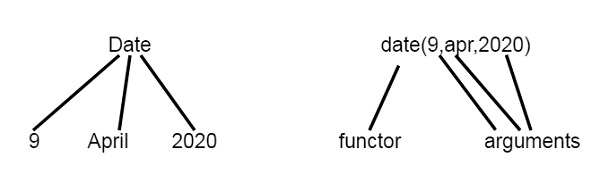
Structures
Structures are Data Objects that contain multiple components.
For example, the date can be viewed as a structure with three components — day, month and year. Then the date 9th April, 2020 can be written as: date(9, apr, 2020).
Note − Structure can in turn have another structure as a component in it.
So we can see views as tree structure and Prolog Functors.
Now let us see one example of structures in Prolog. We will define a structure of points, Segments and Triangle as structures.
To represent a point, a line segment and a triangle using structure in Prolog, we can consider following statements −
-
p1 − point(1, 1)
-
p2 − point(2,3)
-
S − seg( Pl, P2): seg( point(1,1), point(2,3))
-
T − triangle( point(4,Z), point(6,4), point(7,1) )
Note − Structures can be naturally pictured as trees. Prolog can be viewed as a language for processing trees.
Matching in Prolog
Matching is used to check whether two given terms are same (identical) or the variables in both terms can have the same objects after being instantiated. Let us see one example.
Suppose date structure is defined as date(D,M,2020) = date(D1,apr, Y1), this indicates that D = D1, M = feb and Y1 = 2020.
Following rules are to be used to check whether two terms S and T match −
-
If S and T are constants, S=T if both are same objects.
-
If S is a variable and T is anything, T=S.
-
If T is variable and S is anything, S=T.
-
If S and T are structures, S=T if −
-
S and T have same functor.
-
All their corresponding arguments components have to match.
-
Binary Trees
Following is the structure of binary tree using recursive structures −
The definition of the structure is as follows −
node(2, node(1,nil,nil), node(6, node(4,node(3,nil,nil), node(5,nil,nil)), node(7,nil,nil))
Each node has three fields, data and two nodes. One node with no child (leaf node) structure is written as node(value, nil, nil), node with only one left child is written as node(value, left_node, nil), node with only one right child is written as node(value, nil; right_node), and node with both child has node(value, left_node, right_node).
Prolog — Backtracking
In this chapter, we will discuss the backtracking in Prolog. Backtracking is a procedure, in which prolog searches the truth value of different predicates by checking whether they are correct or not. The backtracking term is quite common in algorithm designing, and in different programming environments. In Prolog, until it reaches proper destination, it tries to backtrack. When the destination is found, it stops.
Let us see how backtracking takes place using one tree like structure −
![]()
Suppose A to G are some rules and facts. We start from A and want to reach G. The proper path will be A-C-G, but at first, it will go from A to B, then B to D. When it finds that D is not the destination, it backtracks to B, then go to E, and backtracks again to B, as there is no other child of B, then it backtracks to A, thus it searches for G, and finally found G in the path A-C-G. (Dashed lines are indicating the backtracking.) So when it finds G, it stops.
How Backtracking works?
Now we know, what is the backtracking in Prolog. Let us see one example,
Note − While we are running some prolog code, during backtracking there may be multiple answers, we can press semicolon (;) to get next answers one by one, that helps to backtrack. Otherwise when we get one result, it will stop.
Now, consider a situation, where two people X and Y can pay each other, but the condition is that a boy can pay to a girl, so X will be a boy, and Y will be a girl. So for these we have defined some facts and rules −
Knowledge Base
boy(tom).
boy(bob).
girl(alice).
girl(lili).

pay(X,Y) :- boy(X), girl(Y).
Following is the illustration of the above scenario −
![]()
As X will be a boy, so there are two choices, and for each boy there are two choices alice and lili. Now let us see the output, how backtracking is working.
Output
| ?- [backtrack].
compiling D:/TP Prolog/Sample_Codes/backtrack.pl for byte code...
D:/TP Prolog/Sample_Codes/backtrack.pl compiled, 5 lines read - 703 bytes written, 22 ms

yes
| ?- pay(X,Y).

X = tom
Y = alice ?

(15 ms) yes
| ?- pay(X,Y).

X = tom
Y = alice ? ;

X = tom
Y = lili ? ;

X = bob
Y = alice ? ;

X = bob
Y = lili

yes
| ?- trace.
The debugger will first creep -- showing everything (trace)

(16 ms) yes
{trace}
| ?- pay(X,Y).
   1 1 Call: pay(_23,_24) ?
   2 2 Call: boy(_23) ?
   2 2 Exit: boy(tom) ?
   3 2 Call: girl(_24) ?
   3 2 Exit: girl(alice) ?
   1 1 Exit: pay(tom,alice) ?

X = tom
Y = alice ? ;
   1 1 Redo: pay(tom,alice) ?
   3 2 Redo: girl(alice) ?
   3 2 Exit: girl(lili) ?
   1 1 Exit: pay(tom,lili) ?

X = tom
Y = lili ? ;
   1 1 Redo: pay(tom,lili) ?
   2 2 Redo: boy(tom) ?
   2 2 Exit: boy(bob) ?
   3 2 Call: girl(_24) ?
   3 2 Exit: girl(alice) ?
   1 1 Exit: pay(bob,alice) ?

X = bob
Y = alice ? ;
   1 1 Redo: pay(bob,alice) ?
   3 2 Redo: girl(alice) ?
   3 2 Exit: girl(lili) ?
   1 1 Exit: pay(bob,lili) ?
X = bob
Y = lili

yes
{trace}
| ?-
Preventing Backtracking
So far we have seen some concepts of backtracking. Now let us see some drawbacks of backtracking. Sometimes we write the same predicates more than once when our program demands, for example to write recursive rules or to make some decision making systems. In such cases uncontrolled backtracking may cause inefficiency in a program. To resolve this, we will use the Cut in Prolog.
Suppose we have some rules as follows −
Double step function
-
Rule 1 &minnus; if X < 3 then Y = 0
-
Rule 2 &minnus; if 3 <= X and X < 6 then Y = 2
-
Rule 3 &minnus; if 6 <= X then Y = 4
In Prolog syntax we can write,
-
f(X,0) :- X < 3. % Rule 1
-
f(X,2) :- 3 =< X, X < 6. % Rule 2
-
f(X,4) :- 6 =< X. % Rule 3
Now if we ask for a question as f (1,Y), 2 < Y.
The first goal f(1,Y) instantiated Y to 0. The second goal becomes 2 < 0 which fails. Prolog tries through backtracking two unfruitful alternatives (Rule 2 and Rule 3). If we see closer, we can observe that −
-
The three rules are mutually exclusive and one of them at most will succeed.
-
As soon as one of them succeeds there is no point in trying to use the others as they are bound to fail.
So we can use cut to resolve this. The cut can be expressed using Exclamation symbol. The prolog syntax is as follows −
-
f (X,0) :- X < 3, !. % Rule 1
-
f (X,2) :- 3 =< X, X < 6, !. % Rule 2
-
f (X,4) :- 6 =< X. % Rule 3
Now if we use the same question, ?- f (1,Y), 2 < Y. Prolog choose rule 1 since 1 < 3 and fails the goal 2 < Y fails. Prolog will try to backtrack, but not beyond the point marked ! In the program, rule 2 and rule 3 will not be generated.
Let us see this in below execution −
Program
f(X,0) :- X < 3.              % Rule 1
f(X,2) :- 3 =< X, X < 6.   % Rule 2
f(X,4) :- 6 =< X.             % Rule 3
Output
| ?- [backtrack].
compiling D:/TP Prolog/Sample_Codes/backtrack.pl for byte code...
D:/TP Prolog/Sample_Codes/backtrack.pl compiled, 10 lines read - 1224 bytes written, 17 ms

yes
| ?- f(1,Y), 2<Y.

no
| ?- trace
.
The debugger will first creep -- showing everything (trace)

yes
{trace}
| ?- f(1,Y), 2<Y.
   1 1 Call: f(1,_23) ?
   2 2 Call: 1<3 ?
   2 2 Exit: 1<3 ?
   1 1 Exit: f(1,0) ?
   3 1 Call: 2<0 ?
   3 1 Fail: 2<0 ?
   1 1 Redo: f(1,0) ?
   2 2 Call: 3=<1 ?
   2 2 Fail: 3=<1 ?
   2 2 Call: 6=<1 ?
   2 2 Fail: 6=<1 ?
   1 1 Fail: f(1,_23) ?

(46 ms) no
{trace}
| ?-
Let us see the same using cut.
Program
f(X,0) :- X < 3,!.            % Rule 1
f(X,2) :- 3 =< X, X < 6,!. % Rule 2
f(X,4) :- 6 =< X.             % Rule 3
Output
| ?- [backtrack].
   1 1 Call: [backtrack] ?
compiling D:/TP Prolog/Sample_Codes/backtrack.pl for byte code...
D:/TP Prolog/Sample_Codes/backtrack.pl compiled, 10 lines read - 1373 bytes written, 15 ms
   1 1 Exit: [backtrack] ?
(16 ms) yes
{trace}
| ?- f(1,Y), 2<Y.
   1 1 Call: f(1,_23) ?
   2 2 Call: 1<3 ?
   2 2 Exit: 1<3 ?
   1 1 Exit: f(1,0) ?
   3 1 Call: 2<0 ?
   3 1 Fail: 2<0 ?
no
{trace}
| ?-
Negation as Failure
Here we will perform failure when condition does not satisfy. Suppose we have a statement, “Mary likes all animals but snakes”, we will express this in Prolog.
It would be very easy and straight forward, if the statement is “Mary likes all animals”. In that case we can write “Mary likes X if X is an animal”. And in prolog we can write this statement as, likes(mary, X) := animal(X).
Our actual statement can be expressed as −
-
If X is snake, then “Mary likes X” is not true
-
Otherwise if X is an animal, then Mary likes X.
In prolog we can write this as −
-
likes(mary,X) :- snake(X), !, fail.
-
likes(mary, X) :- animal(X).
The ‘fail’ statement causes the failure. Now let us see how it works in Prolog.
Program
animal(dog).
animal(cat).
animal(elephant).
animal(tiger).
animal(cobra).
animal(python).

snake(cobra).
snake(python).

likes(mary, X) :- snake(X), !, fail.
likes(mary, X) :- animal(X).
Output
| ?- [negate_fail].
compiling D:/TP Prolog/Sample_Codes/negate_fail.pl for byte code...
D:/TP Prolog/Sample_Codes/negate_fail.pl compiled, 11 lines read - 1118 bytes written, 17 ms

yes
| ?- likes(mary,elephant).

yes
| ?- likes(mary,tiger).

yes
| ?- likes(mary,python).

no
| ?- likes(mary,cobra).

no
| ?- trace
.
The debugger will first creep -- showing everything (trace)

yes
{trace}
| ?- likes(mary,dog).
   1 1 Call: likes(mary,dog) ?
   2 2 Call: snake(dog) ?
   2 2 Fail: snake(dog) ?
   2 2 Call: animal(dog) ?
   2 2 Exit: animal(dog) ?
   1 1 Exit: likes(mary,dog) ?

yes
{trace}
| ?- likes(mary,python).
   1 1 Call: likes(mary,python) ?
   2 2 Call: snake(python) ?
   2 2 Exit: snake(python) ?
   3 2 Call: fail ?
   3 2 Fail: fail ?
   1 1 Fail: likes(mary,python) ?

no
{trace}
| ?-
Prolog — Different and Not
Here we will define two predicates — different and not. The different predicate will check whether two given arguments are same or not. If they are same, it will return false, otherwise it will return true. The not predicate is used to negate some statement, which means, when a statement is true, then not(statement) will be false, otherwise if the statement is false, then not(statement) will be true.
So the term ‘different’ can be expressed in three different ways as given below −
-
X and Y are not literally the same
-
X and Y do not match
-
The values of arithmetic expression X and Y are not equal
So in Prolog, we will try to express the statements as follows −
-
If X and Y match, then different(X,Y) fails,
-
Otherwise different(X,Y) succeeds.
The respective prolog syntax will be as follows −
-
different(X, X) :- !, fail.
-
different(X, Y).
We can also express it using disjunctive clauses as given below −
-
different(X, Y) :- X = Y, !, fail ; true. % true is goal that always succeeds
Program
Following example shows how this can be done in prolog −
different(X, X) :- !, fail.
different(X, Y).
Output
| ?- [diff_rel].
compiling D:/TP Prolog/Sample_Codes/diff_rel.pl for byte code...
D:/TP Prolog/Sample_Codes/diff_rel.pl:2: warning: singleton variables [X,Y] for different/2
D:/TP Prolog/Sample_Codes/diff_rel.pl compiled, 2 lines read - 327 bytes written, 11 ms

yes
| ?- different(100,200).

yes
| ?- different(100,100).

no
| ?- different(abc,def).

yes
| ?- different(abc,abc).

no
| ?-
Let us see a program using the disjunctive clauses −
Program
different(X, Y) :- X = Y, !, fail ; true.
Output
| ?- [diff_rel].
compiling D:/TP Prolog/Sample_Codes/diff_rel.pl for byte code...
D:/TP Prolog/Sample_Codes/diff_rel.pl compiled, 0 lines read - 556 bytes written, 17 ms

yes
| ?- different(100,200).

yes
| ?- different(100,100).

no
| ?- different(abc,def).

yes
| ?- different(abc,abc).

no
| ?-
Not Relation in Prolog
The not relation is very much useful in different cases. In our traditional programming languages also, we use the logical not operation to negate some statement. So it means that when a statement is true, then not(statement) will be false, otherwise if the statement is false, then not(statement) will be true.
In prolog, we can define this as shown below −
not(P) :- P, !, fail ; true.
So if P is true, then cut and fail, this will return false, otherwise it will be true. Now let us see one simple code to understand this concept.
Program
not(P) :- P, !, fail ; true.
Output
| ?- [not_rel].
compiling D:/TP Prolog/Sample_Codes/not_rel.pl for byte code...
D:/TP Prolog/Sample_Codes/not_rel.pl compiled, 0 lines read - 630 bytes written, 17 ms

yes
| ?- not(true).

no
| ?- not(fail).

yes
| ?-
Prolog — Inputs and Outputs
In this chapter, we will see some techniques to handle inputs and outputs through prolog. We will use some built in predicates to do these tasks, and also see file handling techniques.
Following topics will be discussed in detail −
-
Handling inputs and outputs
-
File handling using Prolog
-
Using some external file to read lines and terms
-
Character manipulation for input and output
-
Constructing and decomposing atoms
-
Consulting prolog files into other prolog program techniques.
Handling input and output
So far we have seen that we can write a program and the query on the console to execute. In some cases, we print something on the console, that are written in our prolog code. So here we will see that writing and reading tasks in more detail using prolog. So this will be the input and output handling techniques.
The write() Predicate
To write the output we can use the write() predicate. This predicate takes the parameter as input, and writes the content into the console by default. write() can also write in files. Let us see some examples of write() function.
Program
| ?- write(56).
56

yes
| ?- write('hello').
hello

yes
| ?- write('hello'),nl,write('world').
hello
world

yes
| ?- write("ABCDE")
.
[65,66,67,68,69]

yes
From the above example, we can see that the write() predicate can write the contents into the console. We can use ’nl’ to create a new line. And from this example, it is clear that, if we want to print some string on the console, we have to use single quotes (‘string‘). But if we use double quote (“string”), then it will return a list of ASCII values.
The read() Predicate
The read() predicate is used to read from console. User can write something in the console, that can be taken as input and process it. The read() is generally used to read from console, but this can also be used to read from files. Now let us see one example to see how read() works.
Program
cube :-
   write('Write a number: '),
   read(Number),
   process(Number).
process(stop) :- !.
process(Number) :-
   C is Number * Number * Number,
   write('Cube of '),write(Number),write(': '),write(C),nl, cube.
Output
| ?- [read_write].
compiling D:/TP Prolog/Sample_Codes/read_write.pl for byte code...
D:/TP Prolog/Sample_Codes/read_write.pl compiled, 9 lines read - 1226 bytes written, 12 ms

(15 ms) yes
| ?- cube.
Write a number: 2.
Cube of 2: 8
Write a number: 10.
Cube of 10: 1000
Write a number: 12.
Cube of 12: 1728
Write a number: 8.
Cube of 8: 512
Write a number: stop
.

(31 ms) yes
| ?-
The tab() Predicate
The tab() is one additional predicate that can be used to put some blank-spaces while we write something. So it takes a number as an argument, and prints those many number of blank spaces.
Program
| ?- write('hello'),tab(15),write('world').
hello          world

yes
| ?- write('We'),tab(5),write('will'),tab(5),write('use'),tab(5),write('tabs').
We    will  use   tabs

yes
| ?-
Reading/Writing Files
In this section, we will see how we can use files to read from, and write into the files. There are some built-in predicates, that can be used to read from file and write into it.
The tell and told
If we want to write into a file, except the console, we can write the tell() predicate. This tell()predicate takes filename as argument. If that file is not present, then create a new file, and write into it. That file will be opened until we write the told command. We can open more than one file using tell(). When told is called, all files will be closed.
Prolog Commands
| ?- told('myFile.txt').
uncaught exception: error(existence_error(procedure,told/1),top_level/0)
| ?- told("myFile.txt").
uncaught exception: error(existence_error(procedure,told/1),top_level/0)
| ?- tell('myFile.txt').

yes
| ?- tell('myFile.txt').

yes
| ?- write('Hello World').

yes
| ?- write(' Writing into a file'),tab(5),write('myFile.txt'),nl.

yes
| ?- write("Write some ASCII values").

yes
| ?- told.

yes
| ?-
Output (myFile.txt)
Hello World Writing into a file     myFile.txt
[87,114,105,116,101,32,115,111,109,101,32,65,83,67,73,73,32,118,97,108,117,101,115]
Similarly, we can also read from files. Let us see some example of reading from file.
The see and seen
When we want to read from file, not from the keyboard, we have to change current input stream. So we can use see() predicate. This will take filename as input. When the read operation is completed, then we will use seen command.
Sample File (sample_predicate.txt)
likes(lili, cat).
likes(jhon,dog).
Output
| ?- see('sample_predicate.txt'),
read(X),
read(Y),
seen,
read(Z).
the_end.

X = end_of_file
Y = end_of_file
Z = the_end

yes
| ?-
So from this example, we can see that using the see() predicate we can read from the file. Now after using seen command, the control transfers to the console again. So finally it takes input from console.
Processing files of terms
We have seen how to read specific contents (few lines) of a file. Now if we want to read/process all the contents of a file, we need to write a clause to process file (process_file), until we reach the end of the file.
Program
process_file :-
   read(Line),
   Line == end_of_file, % when Line is not not end of file, call process.
   process(Line).
process_file :- !. % use cut to stop backtracking

process(Line):- %this will print the line into the console
   write(Line),nl,
   process_file.
Sample File (sample_predicate.txt)
likes(lili, cat).
likes(jhon,dog).
domestic(dog).
domestic(cat).
Output
| ?- [process_file].
compiling D:/TP Prolog/Sample_Codes/process_file.pl for byte code...
D:/TP Prolog/Sample_Codes/process_file.pl compiled, 9 lines read - 774 bytes written, 23 ms

yes
| ?- see('sample_predicate.txt'), process_file, seen.
likes(lili,cat)
likes(jhon,dog)
domestic(dog)
domestic(cat)

true ?

(15 ms) yes
| ?-
Manipulating characters
Using read() and write() we can read or write the value of atoms, predicates, strings, etc. Now in this section we will see how to write single characters into the current output stream, or how to read from current input stream. So there are some predefined predicates to do these tasks.
The put(C) and put_char(C) predicates
We can use put(C) to write one character at a time into the current output stream. The output stream can be a file or the console. This C can be a character or an ASCII code in other version of Prolog like SWI prolog, but in GNU prolog, it supports only the ASCII value. To use the character instead of ASCII, we can use put_char(C).
Program
| ?- put(97),put(98),put(99),put(100),put(101).
abcde

yes
| ?- put(97),put(66),put(99),put(100),put(101).
aBcde

(15 ms) yes
| ?- put(65),put(66),put(99),put(100),put(101).
ABcde

yes
| ?-put_char('h'),put_char('e'),put_char('l'),put_char('l'),put_char('o').
hello

yes
| ?-
The get_char(C) and get_code(C) predicates
To read a single character from the current input stream, we can use the get_char(C) predicate. This will take the character. if we want the ASCII code, we can use get_code(C).
Program
| ?- get_char(X).
A.

X = 'A'

yes
uncaught exception: error(syntax_error('user_input:6 (char:689) expression expected'),read_term/3)
| ?- get_code(X).
A.

X = 65

yes
uncaught exception: error(syntax_error('user_input:7 (char:14) expression expected'),read_term/3)
| ?-
Constructing Atoms
The atom constructing means from a list of characters, we can make one atom, or from a list of ASCII values also we can make atoms. To do this, we have to use atom_chars() and atom_codes() predicates. In both cases, the first argument will be one variable, and the second argument will be a list. So atom_chars() constructs atom from characters, but atom_codes() construct atoms from ASCII sequence.
Example
| ?- atom_chars(X, ['t','i','g','e','r']).

X = tiger

yes
| ?- atom_chars(A, ['t','o','m']).

A = tom

yes
| ?- atom_codes(X, [97,98,99,100,101]).

X = abcde

yes
| ?- atom_codes(A, [97,98,99]).

A = abc

yes
| ?-
Decomposing Atoms
The atom decomposing means from an atom, we can get a sequence of characters, or a sequence ASCII codes. To do this, we have to use the same atom_chars() and atom_codes() predicates. But one difference is that, in both cases, the first argument will be one atom, and the second argument will be a variable. So atom_chars() decomposes atom to characters, but atom_codes() decomposes atoms to ASCII sequence.
Example
| ?- atom_chars(tiger,X).

X = [t,i,g,e,r]

yes
| ?- atom_chars(tom,A).

A = [t,o,m]

yes
| ?- atom_codes(tiger,X).

X = [116,105,103,101,114]

yes
| ?- atom_codes(tom,A).

A = [116,111,109]

(16 ms) yes
| ?-
The consult in Prolog
The consulting is a technique, that is used to merge the predicates from different files. We can use the consult() predicate, and pass the filename to attach the predicates. Let us see one example program to understand this concept.
Suppose we have two files, namely, prog1.pl and prog2.pl.
Program (prog1.pl)
likes(mary,cat).
likes(joy,rabbit).
likes(tim,duck).
Program (prog2.pl)
likes(suman,mouse).
likes(angshu,deer).
Output
| ?- [prog1].
compiling D:/TP Prolog/Sample_Codes/prog1.pl for byte code...
D:/TP Prolog/Sample_Codes/prog1.pl compiled, 2 lines read - 443 bytes written, 23 ms

yes
| ?- likes(joy,rabbit).

yes
| ?- likes(suman,mouse).

no
| ?- consult('prog2.pl').
compiling D:/TP Prolog/Sample_Codes/prog2.pl for byte code...
D:/TP Prolog/Sample_Codes/prog2.pl compiled, 1 lines read - 366 bytes written, 20 ms
warning: D:/TP Prolog/Sample_Codes/prog2.pl:1: redefining procedure likes/2
         D:/TP Prolog/Sample_Codes/prog1.pl:1: previous definition

yes
| ?- likes(suman,mouse).

yes
| ?- likes(joy,rabbit).

no
| ?-
Now from this output we can understand that this is not as simple as it seems. If two files have completely different clauses, then it will work fine. But if there are same predicates, then while we try to consult the file, it will check the predicates from the second file, when it finds some match, it simply deletes all of the entry of the same predicates from the local database, then load them again from the second file.
Prolog — Built-In Predicates
In Prolog, we have seen the user defined predicates in most of the cases, but there are some built-in-predicates. There are three types of built-in predicates as given below −
-
Identifying terms
-
Decomposing structures
-
Collecting all solutions
So this is the list of some predicates that are falls under the identifying terms group −
| Predicate | Description |
|---|---|
| var(X) | succeeds if X is currently an un-instantiated variable. |
| novar(X) | succeeds if X is not a variable, or already instantiated |
| atom(X) | is true if X currently stands for an atom |
| number(X) | is true if X currently stands for a number |
| integer(X) | is true if X currently stands for an integer |
| float(X) | is true if X currently stands for a real number. |
| atomic(X) | is true if X currently stands for a number or an atom. |
| compound(X) | is true if X currently stands for a structure. |
| ground(X) | succeeds if X does not contain any un-instantiated variables. |
The var(X) Predicate
When X is not initialized, then, it will show true, otherwise false. So let us see an example.
Example
| ?- var(X).

yes
| ?- X = 5, var(X).

no
| ?- var([X]).

no
| ?-
The novar(X) Predicate
When X is not initialized, the, it will show false, otherwise true. So let us see an example.
Example
| ?- nonvar(X).

no
| ?- X = 5,nonvar(X).

X = 5

yes
| ?- nonvar([X]).

yes
| ?-
The atom(X) Predicate
This will return true, when a non-variable term with 0 argument and a not numeric term is passed as X, otherwise false.
Example
| ?- atom(paul).

yes
| ?- X = paul,atom(X).

X = paul

yes
| ?- atom([]).

yes
| ?- atom([a,b]).

no
| ?-
The number(X) Predicate
This will return true, X stands for any number, otherwise false.
Example
| ?- number(X).

no
| ?- X=5,number(X).

X = 5

yes
| ?- number(5.46).

yes
| ?-
The integer(X) Predicate
This will return true, when X is a positive or negative integer value, otherwise false.
Example
| ?- integer(5).

yes
| ?- integer(5.46).

no
| ?-
The float(X) Predicate
This will return true, X is a floating point number, otherwise false.
Example
| ?- float(5).

no
| ?- float(5.46).

yes
| ?-
The atomic(X) Predicate
We have atom(X), that is too specific, it returns false for numeric data, the atomic(X) is like atom(X) but it accepts number.
Example
| ?- atom(5).

no
| ?- atomic(5).

yes
| ?-
The compound(X) Predicate
If atomic(X) fails, then the terms are either one non-instantiated variable (that can be tested with var(X)) or a compound term. Compound will be true when we pass some compound structure.
Example
| ?- compound([]).

no
| ?- compound([a]).

yes
| ?- compound(b(a)).

yes
| ?-
The ground(X) Predicate
This will return true, if X does not contain any un-instantiated variables. This also checks inside the compound terms, otherwise returns false.
Example
| ?- ground(X).

no
| ?- ground(a(b,X)).

no
| ?- ground(a).

yes
| ?- ground([a,b,c]).

yes
| ?-
Decomposing Structures
Now we will see, another group of built-in predicates, that is Decomposing structures. We have seen the identifying terms before. So when we are using compound structures we cannot use a variable to check or make a functor. It will return error. So functor name cannot be represented by a variable.
Error
X = tree, Y = X(maple).
Syntax error Y=X<>(maple)
Now, let us see some inbuilt predicates that falls under the Decomposing structures group.
The functor(T,F,N) Predicate
This returns true if F is the principal functor of T, and N is the arity of F.
Note − Arity means the number of attributes.
Example
| ?- functor(t(f(X),a,T),Func,N).

Func = t
N = 3

(15 ms) yes
| ?-
The arg(N,Term,A) Predicate
This returns true if A is the Nth argument in Term. Otherwise returns false.
Example
| ?- arg(1,t(t(X),[]),A).

A = t(X)

yes
| ?- arg(2,t(t(X),[]),A).

A = []

yes
| ?-
Now, let us see another example. In this example, we are checking that the first argument of D will be 12, the second argument will be apr and the third argument will be 2020.
Example
| ?- functor(D,date,3), arg(1,D,12), arg(2,D,apr), arg(3,D,2020).

D = date(12,apr,2020)

yes
| ?-
The ../2 Predicate
This is another predicate represented as double dot (..). This takes 2 arguments, so ‘/2’ is written. So Term = .. L, this is true if L is a list that contains the functor of Term, followed by its arguments.
Example
| ?- f(a,b) =.. L.

L = [f,a,b]

yes
| ?- T =.. [is_blue,sam,today].

T = is_blue(sam,today)

yes
| ?-
By representing the component of a structure as a list, they can be recursively processed without knowing the functor name. Let us see another example −
Example
| ?- f(2,3)=..[F,N|Y], N1 is N*3, L=..[F,N1|Y].

F = f
L = f(6,3)
N = 2
N1 = 6
Y = [3]

yes
| ?-
Collecting All Solutions
Now let us see the third category called the collecting all solutions, that falls under built-in predicates in Prolog.
We have seen that to generate all of the given solutions of a given goal using the semicolon in the prompt. So here is an example of it.
Example
| ?- member(X, [1,2,3,4]).

X = 1 ? ;

X = 2 ? ;

X = 3 ? ;

X = 4

yes
Sometimes, we need to generate all of the solutions to some goal within a program in some AI related applications. So there are three built-in predicates that will help us to get the results. These predicates are as follows −
-
findall/3
-
setoff/3
-
bagof/3
These three predicates take three arguments, so we have written ‘/3’ after the name of the predicates.
These are also known as meta-predicates. These are used to manipulate Prolog’s Proof strategy.
Syntax
findall(X,P,L).
setof(X,P,L)
bagof(X,P,L)
These three predicates a list of all objects X, such that the goal P is satisfied (example: age(X,Age)). They all repeatedly call the goal P, by instantiating variable X within P and adding it to the list L. This stops when there is no more solution.
Findall/3, Setof/3 and Bagof/3
Here we will see the three different built-in predicates findall/3, setof/3 and the bagof/3, that fall into the category, collecting all solutions.
The findall/3 Predicate
This predicate is used to make a list of all solutions X, from the predicate P. The returned list will be L. So we will read this as “find all of the Xs, such that X is a solution of predicate P and put the list of results in L”. Here this predicate stores the results in the same order, in which Prolog finds them. And if there are duplicate solutions, then all will come into the resultant list, and if there is infinite solution, then the process will never terminate.
Now we can also do some advancement on them. The second argument, which is the goal, that might be a compound goal. Then the syntax will be as findall(X, (Predicate on X, other goal), L)
And also the first argument can be a term of any complexity. So let us see the examples of these few rules, and check the output.
Example
| ?- findall(X, member(X, [1,2,3,4]), Results).

Results = [1,2,3,4]

yes
| ?- findall(X, (member(X, [1,2,3,4]), X > 2), Results).

Results = [3,4]

yes
| ?- findall(X/Y, (member(X,[1,2,3,4]), Y is X * X), Results).

Results = [1/1,2/4,3/9,4/16]

yes
| ?-
The setof/3 Predicate
The setof/3 is also like findall/3, but here it removes all of the duplicate outputs, and the answers will be sorted.
If any variable is used in the goal, then that will not appear in the first argument, setof/3 will return a separate result for each possible instantiation of that variable.
Let us see one example to understand this setof/3. Suppose we have a knowledge base as shown below −
age(peter, 7).
age(ann, 5).
age(pat, 8).
age(tom, 5).
age(ann, 5).
Here we can see that age(ann, 5) has two entries in the knowledge base. And the ages are not sorted, and names are not sorted lexicographically in this case. Now let us see one example of setof/3 usage.
Example
| ?- setof(Child, age(Child,Age),Results).

Age = 5
Results = [ann,tom] ? ;

Age = 7
Results = [peter] ? ;

Age = 8
Results = [pat]

(16 ms) yes
| ?-
Here we can see the ages and the names both are coming sorted. For age 5, there is two entries, so the predicate has created one list corresponding to the age value, with two elements. And the duplicate entry is present only once.
We can use the nested call of setof/3, to collect together the individual results. We will see another example, where the first argument will be Age/Children. As the second argument, it will take another setof like before. So this will return a list of (age/Children) pair. Let us see this in the prolog execution −
Example
| ?- setof(Age/Children, setof(Child,age(Child,Age), Children), AllResults).

AllResults = [5/[ann,tom],7/[peter],8/[pat]]

yes
| ?-
Now if we do not care about a variable that does not appear in the first argument, then we can use the following example −
Example
| ?- setof(Child, Age^age(Child,Age), Results).

Results = [ann,pat,peter,tom]

yes
| ?-
Here we are using the upper caret symbol (^), this indicates that the Age is not in the first argument. So we will read this as, “Find the set of all children, such that the child has an Age (whatever it may be), and put the result in Results”.
The bagof/3 Predicate
The bagof/3 is like setof/3, but here it does not remove the duplicate outputs, and the answers may not be sorted.
Let us see one example to understand this bagof/3. Suppose we have a knowledge base as follows −
Knowledge Base
age(peter, 7).
age(ann, 5).
age(pat, 8).
age(tom, 5).
age(ann, 5).
Example
| ?- bagof(Child, age(Child,Age),Results).

Age = 5
Results = [ann,tom,ann] ? ;

Age = 7
Results = [peter] ? ;

Age = 8
Results = [pat]

(15 ms) yes
| ?-
Here for the Age value 5, the results are [ann, tom, ann]. So the answers are not sorted, and duplicate entries are not removed, so we have got two ‘ann’ values.
The bagof/3 is different from findall/3, as this generates separate results for all the variables in the goal that do not appear in the first argument. We will see this using an example below −
Example
| ?- findall(Child, age(Child,Age),Results).

Results = [peter,ann,pat,tom,ann]

yes
| ?-
Mathematical Predicates
Following are the mathematical predicates −
| Predicates | Description |
|---|---|
| random(L,H,X). | Get random value between L and H |
| between(L,H,X). | Get all values between L and H |
| succ(X,Y). | Add 1 and assign it to X |
| abs(X). | Get absolute value of X |
| max(X,Y). | Get largest value between X and Y |
| min(X,Y). | Get smallest value between X and Y |
| round(X). | Round a value near to X |
| truncate(X). | Convert float to integer, delete the fractional part |
| loor(X). | Round down |
| ceiling(X). | Round up |
| sqrt(X). | Square root |
Besides these, there are some other predicates such as sin, cos, tan, asin, acos, atan, atan2, sinh, cosh, tanh, asinh, acosh, atanh, log, log10, exp, pi, etc.
Now let us see these functions in action using a Prolog program.
Example
| ?- random(0,10,X).

X = 0

yes
| ?- random(0,10,X).

X = 5

yes
| ?- random(0,10,X).

X = 1

yes
| ?- between(0,10,X).

X = 0 ? a

X = 1

X = 2

X = 3

X = 4

X = 5

X = 6

X = 7

X = 8

X = 9

X = 10

(31 ms) yes
| ?- succ(2,X).

X = 3

yes
| ?- X is abs(-8).

X = 8

yes
| ?- X is max(10,5).

X = 10

yes
| ?- X is min(10,5).

X = 5

yes
| ?- X is round(10.56).

X = 11

yes
| ?- X is truncate(10.56).

X = 10

yes
| ?- X is floor(10.56).

X = 10

yes
| ?- X is ceiling(10.56).

X = 11

yes
| ?- X is sqrt(144).

X = 12.0

yes
| ?-
Tree Data Structure (Case Study)
So far we have seen different concepts of logic programming in Prolog. Now we will see one case study on Prolog. We will see how to implement a tree data structure using Prolog, and we will create our own operators. So let us start the planning.
Suppose we have a tree as shown below −

We have to implement this tree using prolog. We have some operations as follows −
-
op(500, xfx, ‘is_parent’).
-
op(500, xfx, ‘is_sibling_of’).
-
op(500, xfx, ‘is_at_same_level’).
-
And another predicate namely leaf_node(Node)
In these operators, you have seen some parameters as (500, xfx, <operator_name>). The first argument (here 500) is the priority of that operator. The ‘xfx’ indicates that this is a binary operator and the <operator_name> is the name of the operator.
These operators can be used to define the tree database. We can use these operators as follows −
-
a is_parent b, or is_parent(a, b). So this indicates that node a is the parent of node b.
-
X is_sibling_of Y or is_sibling_of(X,Y). This indicates that X is the sibling of node Y. So the rule is, if another node Z is parent of X and Z is also the parent of Y and X and Y are different, then X and Y are siblings.
-
leaf_node(Node). A node (Node) is said to be a leaf node when a node has no children.
-
X is_at_same_level Y, or is_at_same_level(X,Y). This will check whether X and Y are at the same level or not. So the condition is when X and Y are same, then it returns true, otherwise W is the parent of X, Z is the parent of Y and W and Z are at the same level.
As shown above, other rules are defined in the code. So let us see the program to get better view.
Program
/* The tree database */

:- op(500,xfx,'is_parent').

a is_parent b. c is_parent g. f is_parent l. j is_parent q.
a is_parent c. c is_parent h. f is_parent m. j is_parent r.
a is_parent d. c is_parent i. h is_parent n. j is_parent s.
b is_parent e. d is_parent j. i is_parent o. m is_parent t.
b is_parent f. e is_parent k. i is_parent p. n is_parent u.
n
is_parent v.
/* X and Y are siblings i.e. child from the same parent */

:- op(500,xfx,'is_sibling_of').

X is_sibling_of Y :- Z is_parent X,
                     Z is_parent Y,
                     X == Y.
leaf_node(Node) :- + is_parent(Node,Child). % Node grounded

/* X and Y are on the same level in the tree. */

:-op(500,xfx,'is_at_same_level').
X is_at_same_level X .
X is_at_same_level Y :- W is_parent X,
                        Z is_parent Y,
                        W is_at_same_level Z.
Output
| ?- [case_tree].
compiling D:/TP Prolog/Sample_Codes/case_tree.pl for byte code...
D:/TP Prolog/Sample_Codes/case_tree.pl:20: warning: singleton variables [Child] for leaf_node/1
D:/TP Prolog/Sample_Codes/case_tree.pl compiled, 28 lines read - 3244 bytes written, 7 ms

yes
| ?- i is_parent p.

yes
| ?- i is_parent s.

no
| ?- is_parent(i,p).

yes
| ?- e is_sibling_of f.

true ?

yes
| ?- is_sibling_of(e,g).

no
| ?- leaf_node(v).

yes
| ?- leaf_node(a).

no
| ?- is_at_same_level(l,s).

true ?

yes
| ?- l is_at_same_level v.

no
| ?-
More on Tree Data Structure
Here, we will see some more operations that will be performed on the above given tree data structure.
Let us consider the same tree here −
We will define other operations −
-
path(Node)
-
locate(Node)
As we have created the last database, we will create a new program that will hold these operations, then consult the new file to use these operations on our pre-existing program.
So let us see what is the purpose of these operators −
-
path(Node) − This will display the path from the root node to the given node. To solve this, suppose X is parent of Node, then find path(X), then write X. When root node ‘a’ is reached, it will stop.
-
locate(Node) − This will locate a node (Node) from the root of the tree. In this case, we will call the path(Node) and write the Node.
Program
Let us see the program in execution −
path(a).                             /* Can start at a. */
path(Node) :- Mother is_parent Node, /* Choose parent, */
              path(Mother),          /* find path and then */
              write(Mother),
              write(' --> ').

/* Locate node by finding a path from root down to the node */
locate(Node) :- path(Node),
                write(Node),
                nl.
Output
| ?- consult('case_tree_more.pl').
compiling D:/TP Prolog/Sample_Codes/case_tree_more.pl for byte code...
D:/TP Prolog/Sample_Codes/case_tree_more.pl compiled, 9 lines read - 866 bytes written, 6 ms

yes
| ?- path(n).
a --> c --> h -->

true ?

yes
| ?- path(s).
a --> d --> j -->

true ?

yes
| ?- path(w).

no
| ?- locate(n).
a --> c --> h --> n

true ?

yes
| ?- locate(s).
a --> d --> j --> s

true ?

yes
| ?- locate(w).

no
| ?-
Advances in Tree Data Structures
Now let us define some advanced operations on the same tree data structure.

Here we will see how to find the height of a node, that is, the length of the longest path from that node, using the Prolog built-in predicate setof/3. This predicate takes (Template, Goal, Set). This binds Set to the list of all instances of Template satisfying the goal Goal.
We have already defined the tree before, so we will consult the current code to execute these set of operations without redefining the tree database again.
We will create some predicates as follows −
ht(Node,H). This finds the height. It also checks whether a node is leaf or not, if so, then sets height H as 0, otherwise recursively finds the height of children of Node, and add 1 to them.
max([X|R], M,A). This calculates the max element from the list, and a value M. So if M is maximum, then it returns M, otherwise, it returns the maximum element of list that is greater than M. To solve this, if given list is empty, return M as max element, otherwise check whether Head is greater than M or not, if so, then call max() using the tail part and the value X, otherwise call max() using tail and the value M.
height(N,H). This uses the setof/3 predicate. This will find the set of results using the goal ht(N,Z) for the template Z and stores into the list type variable called Set. Now find the max of Set, and value 0, store the result into H.
Now let us see the program in execution −
Program
height(N,H) :- setof(Z,ht(N,Z),Set),
               max(Set,0,H).

ht(Node,0) :- leaf_node(Node),!.
ht(Node,H) :- Node is_parent Child,
              ht(Child,H1),
              H is H1 + 1.
max([],M,M).
max([X|R],M,A) :- (X > M -> max(R,X,A) ; max(R,M,A)).
Output
| ?- consult('case_tree_adv.pl').
compiling D:/TP Prolog/Sample_Codes/case_tree_adv.pl for byte code...
D:/TP Prolog/Sample_Codes/case_tree_adv.pl compiled, 9 lines read - 2060 bytes written, 9 ms

yes
| ?- ht(c,H).

H = 1 ? a

H = 3

H = 3

H = 2

H = 2

yes
| ?- max([1,5,3,4,2],10,Max).

Max = 10

yes
| ?- max([1,5,3,40,2],10,Max).

Max = 40

yes
| ?- setof(H, ht(c,H),Set).

Set = [1,2,3]

yes
| ?- max([1,2,3],0,H).

H = 3

yes
| ?- height(c,H).

H = 3

yes
| ?- height(a,H).

H = 4

yes
| ?-
Prolog — Basic Programs
In the following chapter, we are going to discuss basic prolog examples to −
-
Find minimum maximum of two numbers
-
Find the equivalent resistance of a resistive circuit
-
Verify whether a line segment is horizontal, vertical or oblique
Max and Min of two numbers
Here we will see one Prolog program, that can find the minimum of two numbers and the maximum of two numbers. First, we will create two predicates, find_max(X,Y,Max). This takes X and Y values, and stores the maximum value into the Max. Similarly find_min(X,Y,Min) takes X and Y values, and store the minimum value into the Min variable.
Program
find_max(X, Y, X) :- X >= Y, !.
find_max(X, Y, Y) :- X < Y.

find_min(X, Y, X) :- X =< Y, !.
find_min(X, Y, Y) :- X > Y.
Output
| ?- find_max(100,200,Max).

Max = 200

yes
| ?- find_max(40,10,Max).

Max = 40

yes
| ?- find_min(40,10,Min).

Min = 10

yes
| ?- find_min(100,200,Min).

Min = 100

yes
| ?-
Resistance and Resistive Circuits
In this section, we will see how to write a prolog program that will help us find the equivalent resistance of a resistive circuit.
Let us consider the following circuit to understand this concept −
We have to find the equivalent resistance of this network. At first, we will try to get the result by hand, then try to see whether the result is matching with the prolog output or not.
We know that there are two rules −
-
If R1 and R2 are in Series, then equivalent resistor Re = R1 + R2.
-
If R1 and R2 are in Parallel, then equivalent resistor Re = (R1 * R2)/(R1 + R2).
Here 10 Ohm and 40 Ohm resistors are in parallel, then that is in series with 12 Ohm, and the equivalent resistor of the lower half is parallel with 30 Ohm. So let’s try to calculate the equivalent resistance.
-
R3 = (10 * 40)/(10 + 40) = 400/50 = 8 Ohm
-
R4 = R3 + 12 = 8 + 12 = 20 Ohm
-
R5 = (20 * 30)/(20 + 30) = 12 Ohm
Program
series(R1,R2,Re) :- Re is R1 + R2.
parallel(R1,R2,Re) :- Re is ((R1 * R2) / (R1 + R2)).
Output
| ?- [resistance].
compiling D:/TP Prolog/Sample_Codes/resistance.pl for byte code...
D:/TP Prolog/Sample_Codes/resistance.pl compiled, 1 lines read - 804 bytes written, 14 ms

yes
| ?- parallel(10,40,R3).

R3 = 8.0

yes
| ?- series(8,12,R4).

R4 = 20

yes
| ?- parallel(20,30,R5).

R5 = 12.0

yes
| ?- parallel(10,40,R3),series(R3,12,R4),parallel(R4,30,R5).

R3 = 8.0
R4 = 20.0
R5 = 12.0

yes
| ?-
Horizontal and Vertical Line Segments
There are three types of line segments, horizontal, vertical or oblique. This example verifies whether a line segment is horizontal, vertical or oblique.
From this diagram we can understand that −
-
For Horizontal lines, the y coordinate values of two endpoints are same.
-
For Vertical lines, the x coordinate values of two endpoints are same.
-
For Oblique lines, the (x,y) coordinates of two endpoints are different.
Now let us see how to write a program to check this.
Program
vertical(seg(point(X,_),point(X,_))).

horizontal(seg(point(_,Y),point(_,Y))).

oblique(seg(point(X1,Y1),point(X2,Y2)))
   :-X1 == X2,
      Y1 == Y2.
Output
| ?- [line_seg].
compiling D:/TP Prolog/Sample_Codes/line_seg.pl for byte code...
D:/TP Prolog/Sample_Codes/line_seg.pl compiled, 6 lines read - 1276 bytes written, 26 ms

yes
| ?- vertical(seg(point(10,20), point(10,30))).

yes
| ?- vertical(seg(point(10,20), point(15,30))).

no
| ?- oblique(seg(point(10,20), point(15,30))).

yes
| ?- oblique(seg(point(10,20), point(15,20))).

no
| ?- horizontal(seg(point(10,20), point(15,20))).

yes
| ?-
Prolog — Examples of Cuts
In this section, we will see some examples of cuts in prolog. Let us consider, we want to find the maximum of two elements. So we will check these two conditions.
-
If X > Y, then Max := X
-
if X <= Y, then Max := Y
Now from these two lines, we can understand that these two statements are mutually exclusive, so when one is true, another one must be false. In such cases we can use the cut. So let us see the program.
We can also define a predicate where we use the two cases using disjunction (OR logic). So when first one satisfies, it does not check for the second one, otherwise, it will check for the second statement.
Program
max(X,Y,X) :- X >= Y,!.
max(X,Y,Y) :- X < Y.

max_find(X,Y,Max) :- X >= Y,!, Max = X; Max = Y.
Output
| ?- [cut_example].
      1 1 Call: [cut_example] ?
compiling D:/TP Prolog/Sample_Codes/cut_example.pl for byte code...
D:/TP Prolog/Sample_Codes/cut_example.pl compiled, 3 lines read - 1195 bytes written, 43 ms
      1 1 Exit: [cut_example] ?
yes
{trace}
| ?- max(10,20,Max).
      1 1 Call: max(10,20,_23) ?
      2 2 Call: 10>=20 ?
      2 2 Fail: 10>=20 ?
      2 2 Call: 10<20 ?
      2 2 Exit: 10<20 ?
      1 1 Exit: max(10,20,20) ?
Max = 20

yes
{trace}
| ?- max_find(20,10,Max).
      1 1 Call: max_find(20,10,_23) ?
      2 2 Call: 20>=10 ?
      2 2 Exit: 20>=10 ?
      1 1 Exit: max_find(20,10,20) ?
Max = 20

yes
{trace}
| ?-
Program
Let us see another example, where we will use list. In this program we will try to insert an element into a list, if it is not present in the list before. And if the list has the element before we will simply cut it. For the membership checking also, if the item is at the head part, we should not check further, so cut it, otherwise check into the tail part.
list_member(X,[X|_]) :- !.
list_member(X,[_|TAIL]) :- list_member(X,TAIL).

list_append(A,T,T) :- list_member(A,T),!.
list_append(A,T,[A|T]).
Output
| ?- [cut_example].
compiling D:/TP Prolog/Sample_Codes/cut_example.pl for byte code...
D:/TP Prolog/Sample_Codes/cut_example.pl compiled, 9 lines read - 1954 bytes written, 15 ms

yes
| ?- trace.
The debugger will first creep -- showing everything (trace)

yes
{trace}
| ?- list_append(a,[a,b,c,d,e], L).
      1 1 Call: list_append(a,[a,b,c,d,e],_33) ?
      2 2 Call: list_member(a,[a,b,c,d,e]) ?
      2 2 Exit: list_member(a,[a,b,c,d,e]) ?
      1 1 Exit: list_append(a,[a,b,c,d,e],[a,b,c,d,e]) ?

L = [a,b,c,d,e]

yes
{trace}
| ?- list_append(k,[a,b,c,d,e], L).
      1 1 Call: list_append(k,[a,b,c,d,e],_33) ?
      2 2 Call: list_member(k,[a,b,c,d,e]) ?
      3 3 Call: list_member(k,[b,c,d,e]) ?
      4 4 Call: list_member(k,[c,d,e]) ?
      5 5 Call: list_member(k,[d,e]) ?
      6 6 Call: list_member(k,[e]) ?
      7 7 Call: list_member(k,[]) ?
      7 7 Fail: list_member(k,[]) ?
      6 6 Fail: list_member(k,[e]) ?
      5 5 Fail: list_member(k,[d,e]) ?
      4 4 Fail: list_member(k,[c,d,e]) ?
      3 3 Fail: list_member(k,[b,c,d,e]) ?
      2 2 Fail: list_member(k,[a,b,c,d,e]) ?
      1 1 Exit: list_append(k,[a,b,c,d,e],[k,a,b,c,d,e]) ?

L = [k,a,b,c,d,e]

(16 ms) yes
{trace}
| ?-
Prolog — Towers of Hanoi Problem
Towers of Hanoi Problem is a famous puzzle to move N disks from the source peg/tower to the target peg/tower using the intermediate peg as an auxiliary holding peg. There are two conditions that are to be followed while solving this problem −
-
A larger disk cannot be placed on a smaller disk.
-
Only one disk can be moved at a time.
The following diagram depicts the starting setup for N=3 disks.
To solve this, we have to write one procedure move(N, Source, Target, auxiliary). Here N number of disks will have to be shifted from Source peg to Target peg keeping Auxiliary peg as intermediate.
For example – move(3, source, target, auxiliary).
-
Move top disk from source to target
-
Move top disk from source to auxiliary
-
Move top disk from target to auxiliary
-
Move top disk from source to target
-
Move top disk from auxiliary to source
-
Move top disk from auxiliary to target
-
Move top disk from source to target
Program
move(1,X,Y,_) :-
   write('Move top disk from '), write(X), write(' to '), write(Y), nl.
move(N,X,Y,Z) :-
   N>1,
   M is N-1,
   move(M,X,Z,Y),
   move(1,X,Y,_),
   move(M,Z,Y,X).
Output
| ?- [towersofhanoi].
compiling D:/TP Prolog/Sample_Codes/towersofhanoi.pl for byte code...
D:/TP Prolog/Sample_Codes/towersofhanoi.pl compiled, 8 lines read - 1409 bytes written, 15 ms

yes
| ?- move(4,source,target,auxiliary).
Move top disk from source to auxiliary
Move top disk from source to target
Move top disk from auxiliary to target
Move top disk from source to auxiliary
Move top disk from target to source
Move top disk from target to auxiliary
Move top disk from source to auxiliary
Move top disk from source to target
Move top disk from auxiliary to target
Move top disk from auxiliary to source
Move top disk from target to source
Move top disk from auxiliary to target
Move top disk from source to auxiliary
Move top disk from source to target
Move top disk from auxiliary to target

true ?

(31 ms) yes
Prolog — Linked Lists
Following chapters describe how to generate/create linked lists using recursive structures.
Linked list has two components, the integer part and the link part. The link part will hold another node. End of list will have nil into the link part.
In prolog, we can express this using node(2, node(5, node(6, nil))).
Note − The smallest possible list is nil, and every other list will contain nil as the «next» of the end node. In list terminology, the first element is usually called the head of the list, and the rest of the list is called the tail part. Thus the head of the above list is 2, and its tail is the list node(5, node(6, nil)).
We can also insert elements into front and back side −
Program
add_front(L,E,NList) :- NList = node(E,L).

add_back(nil, E, NList) :-
   NList = node(E,nil).

add_back(node(Head,Tail), E, NList) :-
   add_back(Tail, E, NewTail),
   NList = node(Head,NewTail).
Output
| ?- [linked_list].
compiling D:/TP Prolog/Sample_Codes/linked_list.pl for byte code...
D:/TP Prolog/Sample_Codes/linked_list.pl compiled, 7 lines read - 966 bytes written, 14 ms

(15 ms) yes
| ?- add_front(nil, 6, L1), add_front(L1, 5, L2), add_front(L2, 2, L3).

L1 = node(6,nil)
L2 = node(5,node(6,nil))
L3 = node(2,node(5,node(6,nil)))

yes
| ?- add_back(nil, 6, L1), add_back(L1, 5, L2), add_back(L2, 2, L3).

L1 = node(6,nil)
L2 = node(6,node(5,nil))
L3 = node(6,node(5,node(2,nil)))

yes
| ?- add_front(nil, 6, L1), add_front(L1, 5, L2), add_back(L2, 2, L3).

L1 = node(6,nil)
L2 = node(5,node(6,nil))
L3 = node(5,node(6,node(2,nil)))

yes
| ?-
Prolog — Monkey and Banana Problem
In this prolog example, we will see one very interesting and famous problem, The Monkey and Banana Problem.
Problem Statement
Suppose the problem is as given below −
-
A hungry monkey is in a room, and he is near the door.
-
The monkey is on the floor.
-
Bananas have been hung from the center of the ceiling of the room.
-
There is a block (or chair) present in the room near the window.
-
The monkey wants the banana, but cannot reach it.
So how can the monkey get the bananas?
So if the monkey is clever enough, he can come to the block, drag the block to the center, climb on it, and get the banana. Below are few observations in this case −
-
Monkey can reach the block, if both of them are at the same level. From the above image, we can see that both the monkey and the block are on the floor.
-
If the block position is not at the center, then monkey can drag it to the center.
-
If monkey and the block both are on the floor, and block is at the center, then the monkey can climb up on the block. So the vertical position of the monkey will be changed.
-
When the monkey is on the block, and block is at the center, then the monkey can get the bananas.
Now, let us see how we can solve this using Prolog. We will create some predicates as follows −
We have some predicates that will move from one state to another state, by performing action.
-
When the block is at the middle, and monkey is on top of the block, and monkey does not have the banana (i.e. has not state), then using the grasp action, it will change from has not state to have state.
-
From the floor, it can move to the top of the block (i.e. on top state), by performing the action climb.
-
The push or drag operation moves the block from one place to another.
-
Monkey can move from one place to another using walk or move clauses.
Another predicate will be canget(). Here we pass a state, so this will perform move predicate from one state to another using different actions, then perform canget() on state 2. When we have reached to the state ‘has>’, this indicates ‘has banana’. We will stop the execution.
Program
move(state(middle,onbox,middle,hasnot),
   grasp,
   state(middle,onbox,middle,has)).
move(state(P,onfloor,P,H),
   climb,
   state(P,onbox,P,H)).
move(state(P1,onfloor,P1,H),
   drag(P1,P2),
   state(P2,onfloor,P2,H)).
move(state(P1,onfloor,B,H),
   walk(P1,P2),
   state(P2,onfloor,B,H)).
canget(state(_,_,_,has)).
canget(State1) :-
   move(State1,_,State2),
   canget(State2).
Output
| ?- [monkey_banana].
compiling D:/TP Prolog/Sample_Codes/monkey_banana.pl for byte code...
D:/TP Prolog/Sample_Codes/monkey_banana.pl compiled, 17 lines read - 2167 bytes written, 19 ms

(31 ms) yes
| ?- canget(state(atdoor, onfloor, atwindow, hasnot)).

true ?

yes
| ?- trace
.
The debugger will first creep -- showing everything (trace)

yes
{trace}
| ?- canget(state(atdoor, onfloor, atwindow, hasnot)).
      1 1 Call: canget(state(atdoor,onfloor,atwindow,hasnot)) ?
      2 2 Call: move(state(atdoor,onfloor,atwindow,hasnot),_52,_92) ?
      2 2 Exit:move(state(atdoor,onfloor,atwindow,hasnot),walk(atdoor,_80),state(_80,onfloor,atwindow,hasnot)) ?
      3 2 Call: canget(state(_80,onfloor,atwindow,hasnot)) ?
      4 3 Call: move(state(_80,onfloor,atwindow,hasnot),_110,_150) ?
      4 3 Exit: move(state(atwindow,onfloor,atwindow,hasnot),climb,state(atwindow,onbox,atwindow,hasnot)) ?
      5 3 Call: canget(state(atwindow,onbox,atwindow,hasnot)) ?
      6 4 Call: move(state(atwindow,onbox,atwindow,hasnot),_165,_205) ?
      6 4 Fail: move(state(atwindow,onbox,atwindow,hasnot),_165,_193) ?
      5 3 Fail: canget(state(atwindow,onbox,atwindow,hasnot)) ?
      4 3 Redo: move(state(atwindow,onfloor,atwindow,hasnot),climb,state(atwindow,onbox,atwindow,hasnot)) ?
      4 3 Exit: move(state(atwindow,onfloor,atwindow,hasnot),drag(atwindow,_138),state(_138,onfloor,_138,hasnot)) ?
      5 3 Call: canget(state(_138,onfloor,_138,hasnot)) ?
      6 4 Call: move(state(_138,onfloor,_138,hasnot),_168,_208) ?
      6 4 Exit: move(state(_138,onfloor,_138,hasnot),climb,state(_138,onbox,_138,hasnot)) ?
      7 4 Call: canget(state(_138,onbox,_138,hasnot)) ?
      8 5 Call:   move(state(_138,onbox,_138,hasnot),_223,_263) ?
      8 5 Exit: move(state(middle,onbox,middle,hasnot),grasp,state(middle,onbox,middle,has)) ?
      9 5 Call: canget(state(middle,onbox,middle,has)) ?
      9 5 Exit: canget(state(middle,onbox,middle,has)) ?
      7 4 Exit: canget(state(middle,onbox,middle,hasnot)) ?
      5 3 Exit: canget(state(middle,onfloor,middle,hasnot)) ?
      3 2 Exit: canget(state(atwindow,onfloor,atwindow,hasnot)) ?
      1 1 Exit: canget(state(atdoor,onfloor,atwindow,hasnot)) ?

true ?

(78 ms) yes
Prolog — Introduction
Prolog as the name itself suggests, is the short form of LOGical PROgramming. It is a logical and declarative programming language. Before diving deep into the concepts of Prolog, let us first understand what exactly logical programming is.
Logic Programming is one of the Computer Programming Paradigm, in which the program statements express the facts and rules about different problems within a system of formal logic. Here, the rules are written in the form of logical clauses, where head and body are present. For example, H is head and B1, B2, B3 are the elements of the body. Now if we state that “H is true, when B1, B2, B3 all are true”, this is a rule. On the other hand, facts are like the rules, but without any body. So, an example of fact is “H is true”.
Some logic programming languages like Datalog or ASP (Answer Set Programming) are known as purely declarative languages. These languages allow statements about what the program should accomplish. There is no such step-by-step instruction on how to perform the task. However, other languages like Prolog, have declarative and also imperative properties. This may also include procedural statements like “To solve the problem H, perform B1, B2 and B3”.
Some logic programming languages are given below −
-
ALF (algebraic logic functional programming language).
-
ASP (Answer Set Programming)
-
CycL
-
Datalog
-
FuzzyCLIPS
-
Janus
-
Parlog
-
Prolog
-
Prolog++
-
ROOP
Logic and Functional Programming
We will discuss about the differences between Logic programming and the traditional functional programming languages. We can illustrate these two using the below diagram −
From this illustration, we can see that in Functional Programming, we have to define the procedures, and the rule how the procedures work. These procedures work step by step to solve one specific problem based on the algorithm. On the other hand, for the Logic Programming, we will provide knowledge base. Using this knowledge base, the machine can find answers to the given questions, which is totally different from functional programming.
In functional programming, we have to mention how one problem can be solved, but in logic programming we have to specify for which problem we actually want the solution. Then the logic programming automatically finds a suitable solution that will help us solve that specific problem.
Now let us see some more differences below −
| Functional Programming | Logic Programming |
|---|---|
| Functional Programming follows the Von-Neumann Architecture, or uses the sequential steps. | Logic Programming uses abstract model, or deals with objects and their relationships. |
| The syntax is actually the sequence of statements like (a, s, I). | The syntax is basically the logic formulae (Horn Clauses). |
| The computation takes part by executing the statements sequentially. | It computes by deducting the clauses. |
| Logic and controls are mixed together. | Logics and controls can be separated. |
What is Prolog?
Prolog or PROgramming in LOGics is a logical and declarative programming language. It is one major example of the fourth generation language that supports the declarative programming paradigm. This is particularly suitable for programs that involve symbolic or non-numeric computation. This is the main reason to use Prolog as the programming language in Artificial Intelligence, where symbol manipulation and inference manipulation are the fundamental tasks.
In Prolog, we need not mention the way how one problem can be solved, we just need to mention what the problem is, so that Prolog automatically solves it. However, in Prolog we are supposed to give clues as the solution method.
Prolog language basically has three different elements −
Facts − The fact is predicate that is true, for example, if we say, “Tom is the son of Jack”, then this is a fact.
Rules − Rules are extinctions of facts that contain conditional clauses. To satisfy a rule these conditions should be met. For example, if we define a rule as −
grandfather(X, Y) :- father(X, Z), parent(Z, Y)
This implies that for X to be the grandfather of Y, Z should be a parent of Y and X should be father of Z.
Questions − And to run a prolog program, we need some questions, and those questions can be answered by the given facts and rules.
History of Prolog
The heritage of prolog includes the research on theorem provers and some other automated deduction system that were developed in 1960s and 1970s. The Inference mechanism of the Prolog is based on Robinson’s Resolution Principle, that was proposed in 1965, and Answer extracting mechanism by Green (1968). These ideas came together forcefully with the advent of linear resolution procedures.
The explicit goal-directed linear resolution procedures, gave impetus to the development of a general purpose logic programming system. The first Prolog was the Marseille Prolog based on the work by Colmerauer in the year 1970. The manual of this Marseille Prolog interpreter (Roussel, 1975) was the first detailed description of the Prolog language.
Prolog is also considered as a fourth generation programming language supporting the declarative programming paradigm. The well-known Japanese Fifth-Generation Computer Project, that was announced in 1981, adopted Prolog as a development language, and thereby grabbed considerable attention on the language and its capabilities.
Some Applications of Prolog
Prolog is used in various domains. It plays a vital role in automation system. Following are some other important fields where Prolog is used −
-
Intelligent Database Retrieval
-
Natural Language Understanding
-
Specification Language
-
Machine Learning
-
Robot Planning
-
Automation System
-
Problem Solving
Prolog — Environment Setup
In this chapter, we will discuss how to install Prolog in our system.
Prolog Version
In this tutorial, we are using GNU Prolog, Version: 1.4.5
Official Website
This is the official GNU Prolog website where we can see all the necessary details about GNU Prolog, and also get the download link.
http://www.gprolog.org/
Direct Download Link
Given below are the direct download links of GNU Prolog for Windows. For other operating systems like Mac or Linux, you can get the download links by visiting the official website (Link is given above) −
http://www.gprolog.org/setup-gprolog-1.4.5-mingw-x86.exe (32 Bit System)
http://www.gprolog.org/setup-gprolog-1.4.5-mingw-x64.exe(64 Bit System)
Installation Guide
-
Download the exe file and run it.
-
You will see the window as shown below, then click on next −
Select proper directory where you want to install the software, otherwise let it be installed on the default directory. Then click on next.
You will get the below screen, simply go to next.
You can verify the below screen, and check/uncheck appropriate boxes, otherwise you can leave it as default. Then click on next.
In the next step, you will see the below screen, then click on Install.
Then wait for the installation process to finish.
Finally click on Finish to start GNU Prolog.
The GNU prolog is installed successfully as shown below −
Prolog — Hello World
In the previous section, we have seen how to install GNU Prolog. Now, we will see how to write a simple Hello World program in our Prolog environment.
Hello World Program
After running the GNU prolog, we can write hello world program directly from the console. To do so, we have to write the command as follows −
write('Hello World').
Note − After each line, you have to use one period (.) symbol to show that the line has ended.
The corresponding output will be as shown below −
Now let us see how to run the Prolog script file (extension is *.pl) into the Prolog console.
Before running *.pl file, we must store the file into the directory where the GNU prolog console is pointing, otherwise just change the directory by the following steps −
Step 1 − From the prolog console, go to File > Change Dir, then click on that menu.
Step 2 − Select the proper folder and press OK.
Now we can see in the prolog console, it shows that we have successfully changed the directory.
Step 3 − Now create one file (extension is *.pl) and write the code as follows −
main :- write('This is sample Prolog program'),
write(' This program is written into hello_world.pl file').
Now let’s run the code. To run it, we have to write the file name as follows −
[hello_world]
The output is as follows −
Prolog — Basics
In this chapter, we will gain some basic knowledge about Prolog. So we will move on to the first step of our Prolog Programming.
The different topics that will be covered in this chapter are −
Knowledge Base − This is one of the fundamental parts of Logic Programming. We will see in detail about the Knowledge Base, and how it helps in logic programming.
Facts, Rules and Queries − These are the building blocks of logic programming. We will get some detailed knowledge about facts and rules, and also see some kind of queries that will be used in logic programming.
Here, we will discuss about the essential building blocks of logic programming. These building blocks are Facts, Rules and the Queries.
Facts
We can define fact as an explicit relationship between objects, and properties these objects might have. So facts are unconditionally true in nature. Suppose we have some facts as given below −
-
Tom is a cat
-
Kunal loves to eat Pasta
-
Hair is black
-
Nawaz loves to play games
-
Pratyusha is lazy.
So these are some facts, that are unconditionally true. These are actually statements, that we have to consider as true.
Following are some guidelines to write facts −
-
Names of properties/relationships begin with lower case letters.
-
The relationship name appears as the first term.
-
Objects appear as comma-separated arguments within parentheses.
-
A period «.» must end a fact.
-
Objects also begin with lower case letters. They also can begin with digits (like 1234), and can be strings of characters enclosed in quotes e.g. color(penink, ‘red’).
-
phoneno(agnibha, 1122334455). is also called a predicate or clause.
Syntax
The syntax for facts is as follows −
relation(object1,object2...).
Example
Following is an example of the above concept −
cat(tom).
loves_to_eat(kunal,pasta).
of_color(hair,black).
loves_to_play_games(nawaz).
lazy(pratyusha).
Rules
We can define rule as an implicit relationship between objects. So facts are conditionally true. So when one associated condition is true, then the predicate is also true. Suppose we have some rules as given below −
-
Lili is happy if she dances.
-
Tom is hungry if he is searching for food.
-
Jack and Bili are friends if both of them love to play cricket.
-
will go to play if school is closed, and he is free.
So these are some rules that are conditionally true, so when the right hand side is true, then the left hand side is also true.
Here the symbol ( :- ) will be pronounced as “If”, or “is implied by”. This is also known as neck symbol, the LHS of this symbol is called the Head, and right hand side is called Body. Here we can use comma (,) which is known as conjunction, and we can also use semicolon, that is known as disjunction.
Syntax
rule_name(object1, object2, ...) :- fact/rule(object1,
 object2, ...)
Suppose a clause is like :
P :- Q;R.
This can also be written as
P :- Q.
P :- R.

If one clause is like :
P :- Q,R;S,T,U.

Is understood as
P :- (Q,R);(S,T,U).
Or can also be written as:
P :- Q,R.
P :- S,T,U.
Example
happy(lili) :- dances(lili).
hungry(tom) :- search_for_food(tom).
friends(jack, bili) :- lovesCricket(jack), lovesCricket(bili).
goToPlay(ryan) :- isClosed(school), free(ryan).
Queries
Queries are some questions on the relationships between objects and object properties. So question can be anything, as given below −
-
Is tom a cat?
-
Does Kunal love to eat pasta?
-
Is Lili happy?
-
Will Ryan go to play?
So according to these queries, Logic programming language can find the answer and return them.
Knowledge Base in Logic Programming
In this section, we will see what knowledge base in logic programming is.
Well, as we know there are three main components in logic programming − Facts, Rules and Queries. Among these three if we collect the facts and rules as a whole then that forms a Knowledge Base. So we can say that the knowledge base is a collection of facts and rules.
Now, we will see how to write some knowledge bases. Suppose we have our very first knowledge base called KB1. Here in the KB1, we have some facts. The facts are used to state things, that are unconditionally true of the domain of interest.
Knowledge Base 1
Suppose we have some knowledge, that Priya, Tiyasha, and Jaya are three girls, among them, Priya can cook. Let’s try to write these facts in a more generic way as shown below −
girl(priya).
girl(tiyasha).
girl(jaya).
can_cook(priya).
Note − Here we have written the name in lowercase letters, because in Prolog, a string starting with uppercase letter indicates a variable.
Now we can use this knowledge base by posing some queries. “Is priya a girl?”, it will reply “yes”, “is jamini a girl?” then it will answer “No”, because it does not know who jamini is. Our next question is “Can Priya cook?”, it will say “yes”, but if we ask the same question for Jaya, it will say “No”.
Output
GNU Prolog 1.4.5 (64 bits)
Compiled Jul 14 2018, 13:19:42 with x86_64-w64-mingw32-gcc
By Daniel Diaz
Copyright (C) 1999-2018 Daniel Diaz
| ?- change_directory('D:/TP Prolog/Sample_Codes').

yes
| ?- [kb1]
.
compiling D:/TP Prolog/Sample_Codes/kb1.pl for byte code...
D:/TP Prolog/Sample_Codes/kb1.pl compiled, 3 lines read - 489 bytes written, 10 ms

yes
| ?- girl(priya)
.

yes
| ?- girl(jamini).

no
| ?- can_cook(priya).

yes
| ?- can_cook(jaya).

no
| ?-
Let us see another knowledge base, where we have some rules. Rules contain some information that are conditionally true about the domain of interest. Suppose our knowledge base is as follows −
sing_a_song(ananya).
listens_to_music(rohit).

listens_to_music(ananya) :- sing_a_song(ananya).
happy(ananya) :- sing_a_song(ananya).
happy(rohit) :- listens_to_music(rohit).
playes_guitar(rohit) :- listens_to_music(rohit).
So there are some facts and rules given above. The first two are facts, but the rest are rules. As we know that Ananya sings a song, this implies she also listens to music. So if we ask “Does Ananya listen to music?”, the answer will be true. Similarly, “is Rohit happy?”, this will also be true because he listens to music. But if our question is “does Ananya play guitar?”, then according to the knowledge base, it will say “No”. So these are some examples of queries based on this Knowledge base.
Output
| ?- [kb2].
compiling D:/TP Prolog/Sample_Codes/kb2.pl for byte code...
D:/TP Prolog/Sample_Codes/kb2.pl compiled, 6 lines read - 1066 bytes written, 15 ms

yes
| ?- happy(rohit).

yes
| ?- sing_a_song(rohit).

no
| ?- sing_a_song(ananya).

yes
| ?- playes_guitar(rohit).

yes
| ?- playes_guitar(ananya).

no
| ?- listens_to_music(ananya).

yes
| ?-
Knowledge Base 3
The facts and rules of Knowledge Base 3 are as follows −
can_cook(priya).
can_cook(jaya).
can_cook(tiyasha).

likes(priya,jaya) :- can_cook(jaya).
likes(priya,tiyasha) :- can_cook(tiyasha).
Suppose we want to see the members who can cook, we can use one variable in our query. The variables should start with uppercase letters. In the result, it will show one by one. If we press enter, then it will come out, otherwise if we press semicolon (;), then it will show the next result.
Let us see one practical demonstration output to understand how it works.
Output
| ?- [kb3].
compiling D:/TP Prolog/Sample_Codes/kb3.pl for byte code...
D:/TP Prolog/Sample_Codes/kb3.pl compiled, 5 lines read - 737 bytes written, 22 ms
warning: D:/TP Prolog/Sample_Codes/kb3.pl:1: redefining procedure can_cook/1
         D:/TP Prolog/Sample_Codes/kb1.pl:4: previous definition

yes
| ?- can_cook(X).

X = priya ? ;

X = jaya ? ;

X = tiyasha

yes
| ?- likes(priya,X).

X = jaya ? ;

X = tiyasha

yes
| ?-
Prolog — Relations
Relationship is one of the main features that we have to properly mention in Prolog. These relationships can be expressed as facts and rules. After that we will see about the family relationships, how we can express family based relationships in Prolog, and also see the recursive relationships of the family.
We will create the knowledge base by creating facts and rules, and play query on them.
Relations in Prolog
In Prolog programs, it specifies relationship between objects and properties of the objects.
Suppose, there’s a statement, “Amit has a bike”, then we are actually declaring the ownership relationship between two objects — one is Amit and the other is bike.
If we ask a question, “Does Amit own a bike?”, we are actually trying to find out about one relationship.
There are various kinds of relationships, of which some can be rules as well. A rule can find out about a relationship even if the relationship is not defined explicitly as a fact.
We can define a brother relationship as follows −
Two person are brothers, if,
-
They both are male.
-
They have the same parent.
Now consider we have the below phrases −
-
parent(sudip, piyus).
-
parent(sudip, raj).
-
male(piyus).
-
male(raj).
-
brother(X,Y) :- parent(Z,X), parent(Z,Y),male(X), male(Y)
These clauses can give us the answer that piyus and raj are brothers, but we will get three pairs of output here. They are: (piyus, piyus), (piyus, raj), (raj, raj). For these pairs, given conditions are true, but for the pairs (piyus, piyus), (raj, raj), they are not actually brothers, they are the same persons. So we have to create the clauses properly to form a relationship.
The revised relationship can be as follows −
A and B are brothers if −
-
A and B, both are male
-
They have same father
-
They have same mother
-
A and B are not same
Family Relationship in Prolog
Here we will see the family relationship. This is an example of complex relationship that can be formed using Prolog. We want to make a family tree, and that will be mapped into facts and rules, then we can run some queries on them.
Suppose the family tree is as follows −
Here from this tree, we can understand that there are few relationships. Here bob is a child of pam and tom, and bob also has two children — ann and pat. Bob has one brother liz, whose parent is also tom. So we want to make predicates as follows −
Predicates
-
parent(pam, bob).
-
parent(tom, bob).
-
parent(tom, liz).
-
parent(bob, ann).
-
parent(bob, pat).
-
parent(pat, jim).
-
parent(bob, peter).
-
parent(peter, jim).
From our example, it has helped to illustrate some important points −
-
We have defined parent relation by stating the n-tuples of objects based on the given info in the family tree.
-
The user can easily query the Prolog system about relations defined in the program.
-
A Prolog program consists of clauses terminated by a full stop.
-
The arguments of relations can (among other things) be: concrete objects, or constants (such as pat and jim), or general objects such as X and Y. Objects of the first kind in our program are called atoms. Objects of the second kind are called variables.
-
Questions to the system consist of one or more goals.
Some facts can be written in two different ways, like sex of family members can be written in either of the forms −
-
female(pam).
-
male(tom).
-
male(bob).
-
female(liz).
-
female(pat).
-
female(ann).
-
male(jim).
Or in the below form −
-
sex( pam, feminine).
-
sex( tom, masculine).
-
sex( bob, masculine).
-
… and so on.
Now if we want to make mother and sister relationship, then we can write as given below −
In Prolog syntax, we can write −
-
mother(X,Y) :- parent(X,Y), female(X).
-
sister(X,Y) :- parent(Z,X), parent(Z,Y), female(X), X == Y.
Now let us see the practical demonstration −
Knowledge Base (family.pl)
female(pam).
female(liz).
female(pat).
female(ann).
male(jim).
male(bob).
male(tom).
male(peter).
parent(pam,bob).
parent(tom,bob).
parent(tom,liz).
parent(bob,ann).
parent(bob,pat).
parent(pat,jim).
parent(bob,peter).
parent(peter,jim).
mother(X,Y):- parent(X,Y),female(X).
father(X,Y):- parent(X,Y),male(X).
haschild(X):- parent(X,_).
sister(X,Y):- parent(Z,X),parent(Z,Y),female(X),X==Y.
brother(X,Y):-parent(Z,X),parent(Z,Y),male(X),X==Y.
Output
| ?- [family].
compiling D:/TP Prolog/Sample_Codes/family.pl for byte code...
D:/TP Prolog/Sample_Codes/family.pl compiled, 23 lines read - 3088 bytes written, 9 ms

yes
| ?- parent(X,jim).

X = pat ? ;

X = peter

yes
| ?-
mother(X,Y).

X = pam
Y = bob ? ;

X = pat
Y = jim ? ;

no
| ?- haschild(X).

X = pam ? ;

X = tom ? ;

X = tom ? ;

X = bob ? ;

X = bob ? ;

X = pat ? ;

X = bob ? ;

X = peter

yes
| ?- sister(X,Y).

X = liz
Y = bob ? ;

X = ann
Y = pat ? ;

X = ann
Y = peter ? ;

X = pat
Y = ann ? ;

X = pat
Y = peter ? ;

(16 ms) no
| ?-
Now let us see some more relationships that we can make from the previous relationships of a family. So if we want to make a grandparent relationship, that can be formed as follows −
We can also create some other relationships like wife, uncle, etc. We can write the relationships as given below −
-
grandparent(X,Y) :- parent(X,Z), parent(Z,Y).
-
grandmother(X,Z) :- mother(X,Y), parent(Y,Z).
-
grandfather(X,Z) :- father(X,Y), parent(Y,Z).
-
wife(X,Y) :- parent(X,Z),parent(Y,Z), female(X),male(Y).
-
uncle(X,Z) :- brother(X,Y), parent(Y,Z).
So let us write a prolog program to see this in action. Here we will also see the trace to trace-out the execution.
Knowledge Base (family_ext.pl)
female(pam).
female(liz).
female(pat).
female(ann).

male(jim).
male(bob).
male(tom).
male(peter).

parent(pam,bob).
parent(tom,bob).
parent(tom,liz).
parent(bob,ann).

parent(bob,pat).
parent(pat,jim).
parent(bob,peter).
parent(peter,jim).

mother(X,Y):- parent(X,Y),female(X).
father(X,Y):-parent(X,Y),male(X).
sister(X,Y):-parent(Z,X),parent(Z,Y),female(X),X==Y.
brother(X,Y):-parent(Z,X),parent(Z,Y),male(X),X==Y.
grandparent(X,Y):-parent(X,Z),parent(Z,Y).
grandmother(X,Z):-mother(X,Y),parent(Y,Z).
grandfather(X,Z):-father(X,Y),parent(Y,Z).
wife(X,Y):-parent(X,Z),parent(Y,Z),female(X),male(Y).
uncle(X,Z):-brother(X,Y),parent(Y,Z).
Output
| ?- [family_ext].
compiling D:/TP Prolog/Sample_Codes/family_ext.pl for byte code...
D:/TP Prolog/Sample_Codes/family_ext.pl compiled, 27 lines read - 4646 bytes written, 10 ms

| ?- uncle(X,Y).

X = peter
Y = jim ? ;

no
| ?- grandparent(X,Y).

X = pam
Y = ann ? ;

X = pam
Y = pat ? ;

X = pam
Y = peter ? ;

X = tom
Y = ann ? ;

X = tom
Y = pat ? ;

X = tom
Y = peter ? ;

X = bob
Y = jim ? ;

X = bob
Y = jim ? ;

no
| ?- wife(X,Y).

X = pam
Y = tom ? ;

X = pat
Y = peter ? ;

(15 ms) no
| ?-
Tracing the output
In Prolog we can trace the execution. To trace the output, you have to enter into the trace mode by typing “trace.”. Then from the output we can see that we are just tracing “pam is mother of whom?”. See the tracing output by taking X = pam, and Y as variable, there Y will be bob as answer. To come out from the tracing mode press “notrace.”
Program
| ?- [family_ext].
compiling D:/TP Prolog/Sample_Codes/family_ext.pl for byte code...
D:/TP Prolog/Sample_Codes/family_ext.pl compiled, 27 lines read - 4646 bytes written, 10 ms

(16 ms) yes
| ?- mother(X,Y).

X = pam
Y = bob ? ;

X = pat
Y = jim ? ;

no
| ?- trace.
The debugger will first creep -- showing everything (trace)

yes
{trace}
| ?- mother(pam,Y).
   1 1 Call: mother(pam,_23) ?
   2 2 Call: parent(pam,_23) ?
   2 2 Exit: parent(pam,bob) ?
   3 2 Call: female(pam) ?
   3 2 Exit: female(pam) ?
   1 1 Exit: mother(pam,bob) ?

Y = bob

(16 ms) yes
{trace}
| ?- notrace.
The debugger is switched off

yes
| ?-
Recursion in Family Relationship
In the previous section, we have seen that we can define some family relationships. These relationships are static in nature. We can also create some recursive relationships which can be expressed from the following illustration −
So we can understand that predecessor relationship is recursive. We can express this relationship using the following syntax −
predecessor(X, Z) :- parent(X, Z).
predecessor(X, Z) :- parent(X, Y),predecessor(Y, Z).
Now let us see the practical demonstration.
Knowledge Base (family_rec.pl)
female(pam).
female(liz).
female(pat).
female(ann).

male(jim).
male(bob).
male(tom).
male(peter).

parent(pam,bob).
parent(tom,bob).
parent(tom,liz).
parent(bob,ann).
parent(bob,pat).
parent(pat,jim).
parent(bob,peter).
parent(peter,jim).

predecessor(X, Z) :- parent(X, Z).
predecessor(X, Z) :- parent(X, Y),predecessor(Y, Z).
Output
| ?- [family_rec].
compiling D:/TP Prolog/Sample_Codes/family_rec.pl for byte code...
D:/TP Prolog/Sample_Codes/family_rec.pl compiled, 21 lines read - 1851 bytes written, 14 ms

yes
| ?- predecessor(peter,X).

X = jim ? ;

no
| ?- trace.
The debugger will first creep -- showing everything (trace)

yes
{trace}
| ?- predecessor(bob,X).
   1 1 Call: predecessor(bob,_23) ?
   2 2 Call: parent(bob,_23) ?
   2 2 Exit: parent(bob,ann) ?
   1 1 Exit: predecessor(bob,ann) ?

X = ann ? ;
   1 1 Redo: predecessor(bob,ann) ?
   2 2 Redo: parent(bob,ann) ?
   2 2 Exit: parent(bob,pat) ?
   1 1 Exit: predecessor(bob,pat) ?

X = pat ? ;
   1 1 Redo: predecessor(bob,pat) ?
   2 2 Redo: parent(bob,pat) ?
   2 2 Exit: parent(bob,peter) ?
   1 1 Exit: predecessor(bob,peter) ?

X = peter ? ;
   1 1 Redo: predecessor(bob,peter) ?
   2 2 Call: parent(bob,_92) ?
   2 2 Exit: parent(bob,ann) ?
   3 2 Call: predecessor(ann,_23) ?
   4 3 Call: parent(ann,_23) ?
   4 3 Fail: parent(ann,_23) ?
   4 3 Call: parent(ann,_141) ?
   4 3 Fail: parent(ann,_129) ?
   3 2 Fail: predecessor(ann,_23) ?
   2 2 Redo: parent(bob,ann) ?
   2 2 Exit: parent(bob,pat) ?
   3 2 Call: predecessor(pat,_23) ?
   4 3 Call: parent(pat,_23) ?
   4 3 Exit: parent(pat,jim) ?
   3 2 Exit: predecessor(pat,jim) ?
   1 1 Exit: predecessor(bob,jim) ?

X = jim ? ;
   1 1 Redo: predecessor(bob,jim) ?
   3 2 Redo: predecessor(pat,jim) ?
   4 3 Call: parent(pat,_141) ?
   4 3 Exit: parent(pat,jim) ?
   5 3 Call: predecessor(jim,_23) ?
   6 4 Call: parent(jim,_23) ?
   6 4 Fail: parent(jim,_23) ?
   6 4 Call: parent(jim,_190) ?
   6 4 Fail: parent(jim,_178) ?
   5 3 Fail: predecessor(jim,_23) ?
   3 2 Fail: predecessor(pat,_23) ?
   2 2 Redo: parent(bob,pat) ?
   2 2 Exit: parent(bob,peter) ?
   3 2 Call: predecessor(peter,_23) ?
   4 3 Call: parent(peter,_23) ?
   4 3 Exit: parent(peter,jim) ?
   3 2 Exit: predecessor(peter,jim) ?
   1 1 Exit: predecessor(bob,jim) ?

X = jim ?

(78 ms) yes
{trace}
| ?-
Prolog — Data Objects
In this chapter, we will learn data objects in Prolog. They can be divided into few different categories as shown below −
Below are some examples of different kinds of data objects −
-
Atoms − tom, pat, x100, x_45
-
Numbers − 100, 1235, 2000.45
-
Variables − X, Y, Xval, _X
-
Structures − day(9, jun, 2017), point(10, 25)
Atoms and Variables
In this section, we will discuss the atoms, numbers and the variables of Prolog.
Atoms
Atoms are one variation of constants. They can be any names or objects. There are few rules that should be followed when we are trying to use Atoms as given below −
Strings of letters, digits and the underscore character, ‘_’, starting with a lower-case letter. For example −
-
azahar
-
b59
-
b_59
-
b_59AB
-
b_x25
-
antara_sarkar
Strings of special characters
We have to keep in mind that when using atoms of this form, some care is necessary as some strings of special characters already have a predefined meaning; for example ‘:-‘.
-
<—>
-
=======>
-
…
-
.:.
-
::=
Strings of characters enclosed in single quotes.
This is useful if we want to have an atom that starts with a capital letter. By enclosing it in quotes, we make it distinguishable from variables −
-
‘Rubai’
-
‘Arindam_Chatterjee’
-
‘Sumit Mitra’
Numbers
Another variation of constants is the Numbers. So integer numbers can be represented as 100, 4, -81, 1202. In Prolog, the normal range of integers is from -16383 to 16383.
Prolog also supports real numbers, but normally the use-case of floating point number is very less in Prolog programs, because Prolog is for symbolic, non-numeric computation. The treatment of real numbers depends on the implementation of Prolog. Example of real numbers are 3.14159, -0.00062, 450.18, etc.
The variables come under the Simple Objects section. Variables can be used in many such cases in our Prolog program, that we have seen earlier. So there are some rules of defining variables in Prolog.
We can define Prolog variables, such that variables are strings of letters, digits and underscore characters. They start with an upper-case letter or an underscore character. Some examples of Variables are −
-
X
-
Sum
-
Memer_name
-
Student_list
-
Shoppinglist
-
_a50
-
_15
Anonymous Variables in Prolog
Anonymous variables have no names. The anonymous variables in prolog is written by a single underscore character ‘_’. And one important thing is that each individual anonymous variable is treated as different. They are not same.
Now the question is, where should we use these anonymous variables?
Suppose in our knowledge base we have some facts — “jim hates tom”, “pat hates bob”. So if tom wants to find out who hates him, then he can use variables. However, if he wants to check whether there is someone who hates him, we can use anonymous variables. So when we want to use the variable, but do not want to reveal the value of the variable, then we can use anonymous variables.
So let us see its practical implementation −
Knowledge Base (var_anonymous.pl)
hates(jim,tom).
hates(pat,bob).
hates(dog,fox).
hates(peter,tom).
Output
| ?- [var_anonymous].
compiling D:/TP Prolog/Sample_Codes/var_anonymous.pl for byte code...
D:/TP Prolog/Sample_Codes/var_anonymous.pl compiled, 3 lines read - 536 bytes written, 16 ms

yes
| ?- hates(X,tom).

X = jim ? ;

X = peter

yes
| ?- hates(_,tom).

true ? ;

(16 ms) yes
| ?- hates(_,pat).

no
| ?- hates(_,fox).

true ? ;

no
| ?-
Prolog — Operators
In the following sections, we will see what are the different types of operators in Prolog. Types of the comparison operators and Arithmetic operators.
We will also see how these are different from any other high level language operators, how they are syntactically different, and how they are different in their work. Also we will see some practical demonstration to understand the usage of different operators.
Comparison Operators
Comparison operators are used to compare two equations or states. Following are different comparison operators −
| Operator | Meaning |
|---|---|
| X > Y | X is greater than Y |
| X < Y | X is less than Y |
| X >= Y | X is greater than or equal to Y |
| X =< Y | X is less than or equal to Y |
| X =:= Y | the X and Y values are equal |
| X == Y | the X and Y values are not equal |
You can see that the ‘=<’ operator, ‘=:=’ operator and ‘==’ operators are syntactically different from other languages. Let us see some practical demonstration to this.
Example
| ?- 1+2=:=2+1.

yes
| ?- 1+2=2+1.

no
| ?- 1+A=B+2.

A = 2
B = 1

yes
| ?- 5<10.

yes
| ?- 5>10.

no
| ?- 10==100.

yes
Here we can see 1+2=:=2+1 is returning true, but 1+2=2+1 is returning false. This is because, in the first case it is checking whether the value of 1 + 2 is same as 2 + 1 or not, and the other one is checking whether two patterns ‘1+2’ and ‘2+1’ are same or not. As they are not same, it returns no (false). In the case of 1+A=B+2, A and B are two variables, and they are automatically assigned to some values that will match the pattern.
Arithmetic Operators in Prolog
Arithmetic operators are used to perform arithmetic operations. There are few different types of arithmetic operators as follows −
| Operator | Meaning |
|---|---|
| + | Addition |
| — | Subtraction |
| * | Multiplication |
| / | Division |
| ** | Power |
| // | Integer Division |
| mod | Modulus |
Let us see one practical code to understand the usage of these operators.
Program
calc :- X is 100 + 200,write('100 + 200 is '),write(X),nl,
        Y is 400 - 150,write('400 - 150 is '),write(Y),nl,
        Z is 10 * 300,write('10 * 300 is '),write(Z),nl,
        A is 100 / 30,write('100 / 30 is '),write(A),nl,
        B is 100 // 30,write('100 // 30 is '),write(B),nl,
        C is 100 ** 2,write('100 ** 2 is '),write(C),nl,
        D is 100 mod 30,write('100 mod 30 is '),write(D),nl.
Note − The nl is used to create new line.
Output
| ?- change_directory('D:/TP Prolog/Sample_Codes').

yes
| ?- [op_arith].
compiling D:/TP Prolog/Sample_Codes/op_arith.pl for byte code...
D:/TP Prolog/Sample_Codes/op_arith.pl compiled, 6 lines read - 2390 bytes written, 11 ms

yes
| ?- calc.
100 + 200 is 300
400 - 150 is 250
10 * 300 is 3000
100 / 30 is 3.3333333333333335
100 // 30 is 3
100 ** 2 is 10000.0
100 mod 30 is 10

yes
| ?-
Prolog — Loop & Decision Making
In this chapter, we will discuss loops and decision making in Prolog.
Loops
Loop statements are used to execute the code block multiple times. In general, for, while, do-while are loop constructs in programming languages (like Java, C, C++).
Code block is executed multiple times using recursive predicate logic. There are no direct loops in some other languages, but we can simulate loops with few different techniques.
Program
count_to_10(10) :- write(10),nl.
count_to_10(X) :-
   write(X),nl,
   Y is X + 1,
   count_to_10(Y).
Output
| ?- [loop].
compiling D:/TP Prolog/Sample_Codes/loop.pl for byte code...
D:/TP Prolog/Sample_Codes/loop.pl compiled, 4 lines read - 751 bytes written, 16 ms

(16 ms) yes
| ?- count_to_10(3).
3
4
5
6
7
8
9
10

true ?
yes
| ?-
Now create a loop that takes lowest and highest values. So, we can use the between() to simulate loops.
Program
Let us see an example program −
count_down(L, H) :-
   between(L, H, Y),
   Z is H - Y,
   write(Z), nl.

count_up(L, H) :-
   between(L, H, Y),
   Z is L + Y,
   write(Z), nl.
Output
| ?- [loop].
compiling D:/TP Prolog/Sample_Codes/loop.pl for byte code...
D:/TP Prolog/Sample_Codes/loop.pl compiled, 14 lines read - 1700 bytes written, 16 ms

yes
| ?- count_down(12,17).
5

true ? ;
4

true ? ;
3

true ? ;
2

true ? ;
1

true ? ;
0

yes
| ?- count_up(5,12).
10

true ? ;
11

true ? ;
12

true ? ;
13

true ? ;
14

true ? ;
15

true ? ;
16

true ? ;
17

yes
| ?-
Decision Making
The decision statements are If-Then-Else statements. So when we try to match some condition, and perform some task, then we use the decision making statements. The basic usage is as follows −
If <condition> is true, Then <do this>, Else
In some different programming languages, there are If-Else statements, but in Prolog we have to define our statements in some other manner. Following is an example of decision making in Prolog.
Program
% If-Then-Else statement

gt(X,Y) :- X >= Y,write('X is greater or equal').
gt(X,Y) :- X < Y,write('X is smaller').

% If-Elif-Else statement

gte(X,Y) :- X > Y,write('X is greater').
gte(X,Y) :- X =:= Y,write('X and Y are same').
gte(X,Y) :- X < Y,write('X is smaller').
Output
| ?- [test].
compiling D:/TP Prolog/Sample_Codes/test.pl for byte code...
D:/TP Prolog/Sample_Codes/test.pl compiled, 3 lines read - 529 bytes written, 15 ms

yes
| ?- gt(10,100).
X is smaller

yes
| ?- gt(150,100).
X is greater or equal

true ?

yes
| ?- gte(10,20).
X is smaller

(15 ms) yes
| ?- gte(100,20).
X is greater

true ?

yes
| ?- gte(100,100).
X and Y are same

true ?

yes
| ?-
Prolog — Conjunctions & Disjunctions
In this chapter, we shall discuss Conjunction and Disjunction properties. These properties are used in other programming languages using AND and OR logics. Prolog also uses the same logic in its syntax.
Conjunction
Conjunction (AND logic) can be implemented using the comma (,) operator. So two predicates separated by comma are joined with AND statement. Suppose we have a predicate, parent(jhon, bob), which means “Jhon is parent of Bob”, and another predicate, male(jhon), which means “Jhon is male”. So we can make another predicate that father(jhon,bob), which means “Jhon is father of Bob”. We can define predicate father, when he is parent AND he is male.
Disjunction
Disjunction (OR logic) can be implemented using the semi-colon (;) operator. So two predicates separated by semi-colon are joined with OR statement. Suppose we have a predicate, father(jhon, bob). This tells that “Jhon is father of Bob”, and another predicate, mother(lili,bob), this tells that “lili is mother of bob”. If we create another predicate as child(), this will be true when father(jhon, bob) is true OR mother(lili,bob) is true.
Program
parent(jhon,bob).
parent(lili,bob).

male(jhon).
female(lili).

% Conjunction Logic
father(X,Y) :- parent(X,Y),male(X).
mother(X,Y) :- parent(X,Y),female(X).

% Disjunction Logic
child_of(X,Y) :- father(X,Y);mother(X,Y).
Output
| ?- [conj_disj].
compiling D:/TP Prolog/Sample_Codes/conj_disj.pl for byte code...
D:/TP Prolog/Sample_Codes/conj_disj.pl compiled, 11 lines read - 1513 bytes written, 24 ms

yes
| ?- father(jhon,bob).

yes
| ?- child_of(jhon,bob).

true ?

yes
| ?- child_of(lili,bob).

yes
| ?-
Prolog — Lists
In this chapter, we will discuss one of the important concepts in Prolog, The Lists. It is a data structure that can be used in different cases for non-numeric programming. Lists are used to store the atoms as a collection.
In the subsequent sections, we will discuss the following topics −
-
Representation of lists in Prolog
-
Basic operations on prolog such as Insert, delete, update, append.
-
Repositioning operators such as permutation, combination, etc.
-
Set operations like set union, set intersection, etc.
Representation of Lists
The list is a simple data structure that is widely used in non-numeric programming. List consists of any number of items, for example, red, green, blue, white, dark. It will be represented as, [red, green, blue, white, dark]. The list of elements will be enclosed with square brackets.
A list can be either empty or non-empty. In the first case, the list is simply written as a Prolog atom, []. In the second case, the list consists of two things as given below −
-
The first item, called the head of the list;
-
The remaining part of the list, called the tail.
Suppose we have a list like: [red, green, blue, white, dark]. Here the head is red and tail is [green, blue, white, dark]. So the tail is another list.
Now, let us consider we have a list, L = [a, b, c]. If we write Tail = [b, c] then we can also write the list L as L = [ a | Tail]. Here the vertical bar (|) separates the head and tail parts.
So the following list representations are also valid −
-
[a, b, c] = [x | [b, c] ]
-
[a, b, c] = [a, b | [c] ]
-
[a, b, c] = [a, b, c | [ ] ]
For these properties we can define the list as −
A data structure that is either empty or consists of two parts − a head and a tail. The tail itself has to be a list.
Basic Operations on Lists
Following table contains various operations on prolog lists −
| Operations | Definition |
|---|---|
| Membership Checking | During this operation, we can verify whether a given element is member of specified list or not? |
| Length Calculation | With this operation, we can find the length of a list. |
| Concatenation | Concatenation is an operation which is used to join/add two lists. |
| Delete Items | This operation removes the specified element from a list. |
| Append Items | Append operation adds one list into another (as an item). |
| Insert Items | This operation inserts a given item into a list. |
Membership Operation
During this operation, we can check whether a member X is present in list L or not? So how to check this? Well, we have to define one predicate to do so. Suppose the predicate name is list_member(X,L). The goal of this predicate is to check whether X is present in L or not.
To design this predicate, we can follow these observations. X is a member of L if either −
-
X is head of L, or
-
X is a member of the tail of L
Program
list_member(X,[X|_]).
list_member(X,[_|TAIL]) :- list_member(X,TAIL).
Output
| ?- [list_basics].
compiling D:/TP Prolog/Sample_Codes/list_basics.pl for byte code...
D:/TP Prolog/Sample_Codes/list_basics.pl compiled, 1 lines read - 467 bytes written, 13 ms

yes
| ?- list_member(b,[a,b,c]).

true ?

yes
| ?- list_member(b,[a,[b,c]]).

no
| ?- list_member([b,c],[a,[b,c]]).

true ?

yes
| ?- list_member(d,[a,b,c]).

no
| ?- list_member(d,[a,b,c]).
Length Calculation
This is used to find the length of list L. We will define one predicate to do this task. Suppose the predicate name is list_length(L,N). This takes L and N as input argument. This will count the elements in a list L and instantiate N to their number. As was the case with our previous relations involving lists, it is useful to consider two cases −
-
If list is empty, then length is 0.
-
If the list is not empty, then L = [Head|Tail], then its length is 1 + length of Tail.
Program
list_length([],0).
list_length([_|TAIL],N) :- list_length(TAIL,N1), N is N1 + 1.
Output
| ?- [list_basics].
compiling D:/TP Prolog/Sample_Codes/list_basics.pl for byte code...
D:/TP Prolog/Sample_Codes/list_basics.pl compiled, 4 lines read - 985 bytes written, 23 ms

yes
| ?- list_length([a,b,c,d,e,f,g,h,i,j],Len).

Len = 10

yes
| ?- list_length([],Len).

Len = 0

yes
| ?- list_length([[a,b],[c,d],[e,f]],Len).

Len = 3

yes
| ?-
Concatenation
Concatenation of two lists means adding the list items of the second list after the first one. So if two lists are [a,b,c] and [1,2], then the final list will be [a,b,c,1,2]. So to do this task we will create one predicate called list_concat(), that will take first list L1, second list L2, and the L3 as resultant list. There are two observations here.
-
If the first list is empty, and second list is L, then the resultant list will be L.
-
If the first list is not empty, then write this as [Head|Tail], concatenate Tail with L2 recursively, and store into new list in the form, [Head|New List].
Program
list_concat([],L,L).
list_concat([X1|L1],L2,[X1|L3]) :- list_concat(L1,L2,L3).
Output
| ?- [list_basics].
compiling D:/TP Prolog/Sample_Codes/list_basics.pl for byte code...
D:/TP Prolog/Sample_Codes/list_basics.pl compiled, 7 lines read - 1367 bytes written, 19 ms

yes
| ?- list_concat([1,2],[a,b,c],NewList).

NewList = [1,2,a,b,c]

yes
| ?- list_concat([],[a,b,c],NewList).

NewList = [a,b,c]

yes
| ?- list_concat([[1,2,3],[p,q,r]],[a,b,c],NewList).

NewList = [[1,2,3],[p,q,r],a,b,c]

yes
| ?-
Delete from List
Suppose we have a list L and an element X, we have to delete X from L. So there are three cases −
-
If X is the only element, then after deleting it, it will return empty list.
-
If X is head of L, the resultant list will be the Tail part.
-
If X is present in the Tail part, then delete from there recursively.
Program
list_delete(X, [X], []).
list_delete(X,[X|L1], L1).
list_delete(X, [Y|L2], [Y|L1]) :- list_delete(X,L2,L1).
Output
| ?- [list_basics].
compiling D:/TP Prolog/Sample_Codes/list_basics.pl for byte code...
D:/TP Prolog/Sample_Codes/list_basics.pl compiled, 11 lines read - 1923 bytes written, 25 ms

yes
| ?- list_delete(a,[a,e,i,o,u],NewList).

NewList = [e,i,o,u] ?

yes
| ?- list_delete(a,[a],NewList).

NewList = [] ?

yes
| ?- list_delete(X,[a,e,i,o,u],[a,e,o,u]).

X = i ? ;

no
| ?-
Append into List
Appending two lists means adding two lists together, or adding one list as an item. Now if the item is present in the list, then the append function will not work. So we will create one predicate namely, list_append(L1, L2, L3). The following are some observations −
-
Let A is an element, L1 is a list, the output will be L1 also, when L1 has A already.
-
Otherwise new list will be L2 = [A|L1].
Program
list_member(X,[X|_]).
list_member(X,[_|TAIL]) :- list_member(X,TAIL).

list_append(A,T,T) :- list_member(A,T),!.
list_append(A,T,[A|T]).
In this case, we have used (!) symbol, that is known as cut. So when the first line is executed successfully, then we cut it, so it will not execute the next operation.
Output
| ?- [list_basics].
compiling D:/TP Prolog/Sample_Codes/list_basics.pl for byte code...
D:/TP Prolog/Sample_Codes/list_basics.pl compiled, 14 lines read - 2334 bytes written, 25 ms

(16 ms) yes
| ?- list_append(a,[e,i,o,u],NewList).

NewList = [a,e,i,o,u]

yes
| ?- list_append(e,[e,i,o,u],NewList).

NewList = [e,i,o,u]

yes
| ?- list_append([a,b],[e,i,o,u],NewList).

NewList = [[a,b],e,i,o,u]

yes
| ?-
Insert into List
This method is used to insert an item X into list L, and the resultant list will be R. So the predicate will be in this form list_insert(X, L, R). So this can insert X into L in all possible positions. If we see closer, then there are some observations.
-
If we perform list_insert(X,L,R), we can use list_delete(X,R,L), so delete X from R and make new list L.
Program
list_delete(X, [X], []).
list_delete(X,[X|L1], L1).
list_delete(X, [Y|L2], [Y|L1]) :- list_delete(X,L2,L1).

list_insert(X,L,R) :- list_delete(X,R,L).
Output
| ?- [list_basics].
compiling D:/TP Prolog/Sample_Codes/list_basics.pl for byte code...
D:/TP Prolog/Sample_Codes/list_basics.pl compiled, 16 lines read - 2558 bytes written, 22 ms

(16 ms) yes
| ?- list_insert(a,[e,i,o,u],NewList).

NewList = [a,e,i,o,u] ? a

NewList = [e,a,i,o,u]

NewList = [e,i,a,o,u]

NewList = [e,i,o,a,u]

NewList = [e,i,o,u,a]

NewList = [e,i,o,u,a]

(15 ms) no
| ?-
Repositioning operations of list items
Following are repositioning operations −
| Repositioning Operations | Definition |
|---|---|
| Permutation | This operation will change the list item positions and generate all possible outcomes. |
| Reverse Items | This operation arranges the items of a list in reverse order. |
| Shift Items | This operation will shift one element of a list to the left rotationally. |
| Order Items | This operation verifies whether the given list is ordered or not. |
Permutation Operation
This operation will change the list item positions and generate all possible outcomes. So we will create one predicate as list_perm(L1,L2), This will generate all permutation of L1, and store them into L2. To do this we need list_delete() clause to help.
To design this predicate, we can follow few observations as given below −
X is member of L if either −
-
If the first list is empty, then the second list must also be empty.
-
If the first list is not empty then it has the form [X | L], and a permutation of such a list can be constructed as, first permute L obtaining L1 and then insert X at any position into L1.
Program
list_delete(X,[X|L1], L1).
list_delete(X, [Y|L2], [Y|L1]) :- list_delete(X,L2,L1).

list_perm([],[]).
list_perm(L,[X|P]) :- list_delete(X,L,L1),list_perm(L1,P).
Output
| ?- [list_repos].
compiling D:/TP Prolog/Sample_Codes/list_repos.pl for byte code...
D:/TP Prolog/Sample_Codes/list_repos.pl compiled, 4 lines read - 1060 bytes written, 17 ms

(15 ms) yes
| ?- list_perm([a,b,c,d],X).

X = [a,b,c,d] ? a

X = [a,b,d,c]

X = [a,c,b,d]

X = [a,c,d,b]

X = [a,d,b,c]

X = [a,d,c,b]

X = [b,a,c,d]

X = [b,a,d,c]

X = [b,c,a,d]

X = [b,c,d,a]

X = [b,d,a,c]

X = [b,d,c,a]

X = [c,a,b,d]

X = [c,a,d,b]

X = [c,b,a,d]

X = [c,b,d,a]

X = [c,d,a,b]

X = [c,d,b,a]

X = [d,a,b,c]

X = [d,a,c,b]

X = [d,b,a,c]

X = [d,b,c,a]

X = [d,c,a,b]

X = [d,c,b,a]

(31 ms) no
| ?-
Reverse Operation
Suppose we have a list L = [a,b,c,d,e], and we want to reverse the elements, so the output will be [e,d,c,b,a]. To do this, we will create a clause, list_reverse(List, ReversedList). Following are some observations −
-
If the list is empty, then the resultant list will also be empty.
-
Otherwise put the list items namely, [Head|Tail], and reverse the Tail items recursively, and concatenate with the Head.
-
Otherwise put the list items namely, [Head|Tail], and reverse the Tail items recursively, and concatenate with the Head.
Program
list_concat([],L,L).
list_concat([X1|L1],L2,[X1|L3]) :- list_concat(L1,L2,L3).

list_rev([],[]).
list_rev([Head|Tail],Reversed) :-
   list_rev(Tail, RevTail),list_concat(RevTail, [Head],Reversed).
Output
| ?- [list_repos].
compiling D:/TP Prolog/Sample_Codes/list_repos.pl for byte code...
D:/TP Prolog/Sample_Codes/list_repos.pl compiled, 10 lines read - 1977 bytes written, 19 ms

yes
| ?- list_rev([a,b,c,d,e],NewList).

NewList = [e,d,c,b,a]

yes
| ?- list_rev([a,b,c,d,e],[e,d,c,b,a]).

yes
| ?-
Shift Operation
Using Shift operation, we can shift one element of a list to the left rotationally. So if the list items are [a,b,c,d], then after shifting, it will be [b,c,d,a]. So we will make a clause list_shift(L1, L2).
-
We will express the list as [Head|Tail], then recursively concatenate Head after the Tail, so as a result we can feel that the elements are shifted.
-
This can also be used to check whether the two lists are shifted at one position or not.
Program
list_concat([],L,L).
list_concat([X1|L1],L2,[X1|L3]) :- list_concat(L1,L2,L3).

list_shift([Head|Tail],Shifted) :- list_concat(Tail, [Head],Shifted).
Output
| ?- [list_repos].
compiling D:/TP Prolog/Sample_Codes/list_repos.pl for byte code...
D:/TP Prolog/Sample_Codes/list_repos.pl compiled, 12 lines read - 2287 bytes written, 10 ms

yes
| ?- list_shift([a,b,c,d,e],L2).

L2 = [b,c,d,e,a]

(16 ms) yes
| ?- list_shift([a,b,c,d,e],[b,c,d,e,a]).

yes
| ?-
Order Operation
Here we will define a predicate list_order(L) which checks whether L is ordered or not. So if L = [1,2,3,4,5,6], then the result will be true.
-
If there is only one element, that is already ordered.
-
Otherwise take first two elements X and Y as Head, and rest as Tail. If X =< Y, then call the clause again with the parameter [Y|Tail], so this will recursively check from the next element.
Program
list_order([X, Y | Tail]) :- X =< Y, list_order([Y|Tail]).
list_order([X]).
Output
| ?- [list_repos]. compiling D:/TP Prolog/Sample_Codes/list_repos.pl for byte code... D:/TP Prolog/Sample_Codes/list_repos.pl:15: warning: singleton variables [X] for list_order/1 D:/TP Prolog/Sample_Codes/list_repos.pl compiled, 15 lines read - 2805 bytes written, 18 ms yes | ?- list_order([1,2,3,4,5,6,6,7,7,8]). true ? yes | ?- list_order([1,4,2,3,6,5]). no | ?-
Set operations on lists
We will try to write a clause that will get all possible subsets of a given set. So if the set is [a,b], then the result will be [], [a], [b], [a,b]. To do so, we will create one clause, list_subset(L, X). It will take L and return each subsets into X. So we will proceed in the following way −
-
If list is empty, the subset is also empty.
-
Find the subset recursively by retaining the Head, and
-
Make another recursive call where we will remove Head.
Program
list_subset([],[]). list_subset([Head|Tail],[Head|Subset]) :- list_subset(Tail,Subset). list_subset([Head|Tail],Subset) :- list_subset(Tail,Subset).
Output
| ?- [list_set]. compiling D:/TP Prolog/Sample_Codes/list_set.pl for byte code... D:/TP Prolog/Sample_Codes/list_set.pl:3: warning: singleton variables [Head] for list_subset/2 D:/TP Prolog/Sample_Codes/list_set.pl compiled, 2 lines read - 653 bytes written, 7 ms yes | ?- list_subset([a,b],X). X = [a,b] ? ; X = [a] ? ; X = [b] ? ; X = [] (15 ms) yes | ?- list_subset([x,y,z],X). X = [x,y,z] ? a X = [x,y] X = [x,z] X = [x] X = [y,z] X = [y] X = [z] X = [] yes | ?-
Union Operation
Let us define a clause called list_union(L1,L2,L3), So this will take L1 and L2, and perform Union on them, and store the result into L3. As you know if two lists have the same element twice, then after union, there will be only one. So we need another helper clause to check the membership.
Program
list_member(X,[X|_]). list_member(X,[_|TAIL]) :- list_member(X,TAIL). list_union([X|Y],Z,W) :- list_member(X,Z),list_union(Y,Z,W). list_union([X|Y],Z,[X|W]) :- + list_member(X,Z), list_union(Y,Z,W). list_union([],Z,Z).
Note − In the program, we have used (+) operator, this operator is used for NOT.
Output
| ?- [list_set]. compiling D:/TP Prolog/Sample_Codes/list_set.pl for byte code... D:/TP Prolog/Sample_Codes/list_set.pl:6: warning: singleton variables [Head] for list_subset/2 D:/TP Prolog/Sample_Codes/list_set.pl compiled, 9 lines read - 2004 bytes written, 18 ms yes | ?- list_union([a,b,c,d,e],[a,e,i,o,u],L3). L3 = [b,c,d,a,e,i,o,u] ? (16 ms) yes | ?- list_union([a,b,c,d,e],[1,2],L3). L3 = [a,b,c,d,e,1,2] yes
Intersection Operation
Let us define a clause called list_intersection(L1,L2,L3), So this will take L1 and L2, and perform Intersection operation, and store the result into L3. Intersection will return those elements that are present in both lists. So L1 = [a,b,c,d,e], L2 = [a,e,i,o,u], then L3 = [a,e]. Here, we will use the list_member() clause to check if one element is present in a list or not.
Program
list_member(X,[X|_]). list_member(X,[_|TAIL]) :- list_member(X,TAIL). list_intersect([X|Y],Z,[X|W]) :- list_member(X,Z), list_intersect(Y,Z,W). list_intersect([X|Y],Z,W) :- + list_member(X,Z), list_intersect(Y,Z,W). list_intersect([],Z,[]).
Output
| ?- [list_set]. compiling D:/TP Prolog/Sample_Codes/list_set.pl for byte code... D:/TP Prolog/Sample_Codes/list_set.pl compiled, 13 lines read - 3054 bytes written, 9 ms (15 ms) yes | ?- list_intersect([a,b,c,d,e],[a,e,i,o,u],L3). L3 = [a,e] ? yes | ?- list_intersect([a,b,c,d,e],[],L3). L3 = [] yes | ?-
Misc Operations on Lists
Following are some miscellaneous operations that can be performed on lists −
| Misc Operations | Definition |
|---|---|
| Even and Odd Length Finding | Verifies whether the list has odd number or even number of elements. |
| Divide | Divides a list into two lists, and these lists are of approximately same length. |
| Max | Retrieves the element with maximum value from the given list. |
| Sum | Returns the sum of elements of the given list. |
| Merge Sort | Arranges the elements of a given list in order (using Merge Sort algorithm). |
Even and Odd Length Operation
In this example, we will see two operations using which we can check whether the list has odd number of elements or the even number of elements. We will define predicates namely, list_even_len(L) and list_odd_len(L).
-
If the list has no elements, then that is even length list.
-
Otherwise we take it as [Head|Tail], then if Tail is of odd length, then the total list is even length string.
-
Similarly, if the list has only one element, then that is odd length list.
-
By taking it as [Head|Tail] and Tail is even length string, then entire list is odd length list.
Program
list_even_len([]). list_even_len([Head|Tail]) :- list_odd_len(Tail). list_odd_len([_]). list_odd_len([Head|Tail]) :- list_even_len(Tail).
Output
| ?- [list_misc]. compiling D:/TP Prolog/Sample_Codes/list_misc.pl for byte code... D:/TP Prolog/Sample_Codes/list_misc.pl:2: warning: singleton variables [Head] for list_even_len/1 D:/TP Prolog/Sample_Codes/list_misc.pl:5: warning: singleton variables [Head] for list_odd_len/1 D:/TP Prolog/Sample_Codes/list_misc.pl compiled, 4 lines read - 726 bytes written, 20 ms yes | ?- list_odd_len([a,2,b,3,c]). true ? yes | ?- list_odd_len([a,2,b,3]). no | ?- list_even_len([a,2,b,3]). true ? yes | ?- list_even_len([a,2,b,3,c]). no | ?-
Divide List Operation
This operation divides a list into two lists, and these lists are of approximately same length. So if the given list is [a,b,c,d,e], then the result will be [a,c,e],[b,d]. This will place all of the odd placed elements into one list, and all even placed elements into another list. We will define a predicate, list_divide(L1,L2,L3) to solve this task.
-
If given list is empty, then it will return empty lists.
-
If there is only one element, then the first list will be a list with that element, and the second list will be empty.
-
Suppose X,Y are two elements from head, and rest are Tail, So make two lists [X|List1], [Y|List2], these List1 and List2 are separated by dividing Tail.
Program
list_divide([],[],[]). list_divide([X],[X],[]). list_divide([X,Y|Tail], [X|List1],[Y|List2]) :- list_divide(Tail,List1,List2).
Output
| ?- [list_misc]. compiling D:/TP Prolog/Sample_Codes/list_misc.pl for byte code... D:/TP Prolog/Sample_Codes/list_misc.pl:2: warning: singleton variables [Head] for list_even_len/1 D:/TP Prolog/Sample_Codes/list_misc.pl:5: warning: singleton variables [Head] for list_odd_len/1 D:/TP Prolog/Sample_Codes/list_misc.pl compiled, 8 lines read - 1432 bytes written, 8 ms yes | ?- list_divide([a,1,b,2,c,3,d,5,e],L1,L2). L1 = [a,b,c,d,e] L2 = [1,2,3,5] ? yes | ?- list_divide([a,b,c,d],L1,L2). L1 = [a,c] L2 = [b,d] yes | ?-
Max Item Operation
This operation is used to find the maximum element from a list. We will define a predicate, list_max_elem(List, Max), then this will find Max element from the list and return.
-
If there is only one element, then it will be the max element.
-
Divide the list as [X,Y|Tail]. Now recursively find max of [Y|Tail] and store it into MaxRest, and store maximum of X and MaxRest, then store it to Max.
Program
max_of_two(X,Y,X) :- X >= Y. max_of_two(X,Y,Y) :- X < Y. list_max_elem([X],X). list_max_elem([X,Y|Rest],Max) :- list_max_elem([Y|Rest],MaxRest), max_of_two(X,MaxRest,Max).
Output
| ?- [list_misc]. compiling D:/TP Prolog/Sample_Codes/list_misc.pl for byte code... D:/TP Prolog/Sample_Codes/list_misc.pl:2: warning: singleton variables [Head] for list_even_len/1 D:/TP Prolog/Sample_Codes/list_misc.pl:5: warning: singleton variables [Head] for list_odd_len/1 D:/TP Prolog/Sample_Codes/list_misc.pl compiled, 16 lines read - 2385 bytes written, 16 ms yes | ?- list_max_elem([8,5,3,4,7,9,6,1],Max). Max = 9 ? yes | ?- list_max_elem([5,12,69,112,48,4],Max). Max = 112 ? yes | ?-
List Sum Operation
In this example, we will define a clause, list_sum(List, Sum), this will return the sum of the elements of the list.
-
If the list is empty, then sum will be 0.
-
Represent list as [Head|Tail], find sum of tail recursively and store them into SumTemp, then set Sum = Head + SumTemp.
Program
list_sum([],0). list_sum([Head|Tail], Sum) :- list_sum(Tail,SumTemp), Sum is Head + SumTemp.
Output
yes | ?- [list_misc]. compiling D:/TP Prolog/Sample_Codes/list_misc.pl for byte code... D:/TP Prolog/Sample_Codes/list_misc.pl:2: warning: singleton variables [Head] for list_even_len/1 D:/TP Prolog/Sample_Codes/list_misc.pl:5: warning: singleton variables [Head] for list_odd_len/1 D:/TP Prolog/Sample_Codes/list_misc.pl compiled, 21 lines read - 2897 bytes written, 21 ms (32 ms) yes | ?- list_sum([5,12,69,112,48,4],Sum). Sum = 250 yes | ?- list_sum([8,5,3,4,7,9,6,1],Sum). Sum = 43 yes | ?-
Merge Sort on a List
If the list is [4,5,3,7,8,1,2], then the result will be [1,2,3,4,5,7,8]. The steps of performing merge sort are shown below −
-
Take the list and split them into two sub-lists. This split will be performed recursively.
-
Merge each split in sorted order.
-
Thus the entire list will be sorted.
We will define a predicate called mergesort(L, SL), it will take L and return result into SL.
Program
mergesort([],[]). /* covers special case */ mergesort([A],[A]). mergesort([A,B|R],S) :- split([A,B|R],L1,L2), mergesort(L1,S1), mergesort(L2,S2), merge(S1,S2,S). split([],[],[]). split([A],[A],[]). split([A,B|R],[A|Ra],[B|Rb]) :- split(R,Ra,Rb). merge(A,[],A). merge([],B,B). merge([A|Ra],[B|Rb],[A|M]) :- A =< B, merge(Ra,[B|Rb],M). merge([A|Ra],[B|Rb],[B|M]) :- A > B, merge([A|Ra],Rb,M).
Output
| ?- [merge_sort]. compiling D:/TP Prolog/Sample_Codes/merge_sort.pl for byte code... D:/TP Prolog/Sample_Codes/merge_sort.pl compiled, 17 lines read - 3048 bytes written, 19 ms yes | ?- mergesort([4,5,3,7,8,1,2],L). L = [1,2,3,4,5,7,8] ? yes | ?- mergesort([8,5,3,4,7,9,6,1],L). L = [1,3,4,5,6,7,8,9] ? yes | ?-
Prolog — Recursion and Structures
This chapter covers recursion and structures.
Recursion
Recursion is a technique in which one predicate uses itself (may be with some other predicates) to find the truth value.
Let us understand this definition with the help of an example −
-
is_digesting(X,Y) :- just_ate(X,Y).
-
is_digesting(X,Y) :-just_ate(X,Z),is_digesting(Z,Y).
So this predicate is recursive in nature. Suppose we say that just_ate(deer, grass), it means is_digesting(deer, grass) is true. Now if we say is_digesting(tiger, grass), this will be true if is_digesting(tiger, grass) :- just_ate(tiger, deer), is_digesting(deer, grass), then the statement is_digesting(tiger, grass) is also true.
There may be some other examples also, so let us see one family example. So if we want to express the predecessor logic, that can be expressed using the following diagram −
So we can understand the predecessor relationship is recursive. We can express this relationship using the following syntax −
-
predecessor(X, Z) :- parent(X, Z).
-
predecessor(X, Z) :- parent(X, Y),predecessor(Y, Z).
Structures
Structures are Data Objects that contain multiple components.
For example, the date can be viewed as a structure with three components — day, month and year. Then the date 9th April, 2020 can be written as: date(9, apr, 2020).
Note − Structure can in turn have another structure as a component in it.
So we can see views as tree structure and Prolog Functors.
Now let us see one example of structures in Prolog. We will define a structure of points, Segments and Triangle as structures.
To represent a point, a line segment and a triangle using structure in Prolog, we can consider following statements −
-
p1 − point(1, 1)
-
p2 − point(2,3)
-
S − seg( Pl, P2): seg( point(1,1), point(2,3))
-
T − triangle( point(4,Z), point(6,4), point(7,1) )
Note − Structures can be naturally pictured as trees. Prolog can be viewed as a language for processing trees.
Matching in Prolog
Matching is used to check whether two given terms are same (identical) or the variables in both terms can have the same objects after being instantiated. Let us see one example.
Suppose date structure is defined as date(D,M,2020) = date(D1,apr, Y1), this indicates that D = D1, M = feb and Y1 = 2020.
Following rules are to be used to check whether two terms S and T match −
-
If S and T are constants, S=T if both are same objects.
-
If S is a variable and T is anything, T=S.
-
If T is variable and S is anything, S=T.
-
If S and T are structures, S=T if −
-
S and T have same functor.
-
All their corresponding arguments components have to match.
-
Binary Trees
Following is the structure of binary tree using recursive structures −
The definition of the structure is as follows −
node(2, node(1,nil,nil), node(6, node(4,node(3,nil,nil), node(5,nil,nil)), node(7,nil,nil))
Each node has three fields, data and two nodes. One node with no child (leaf node) structure is written as node(value, nil, nil), node with only one left child is written as node(value, left_node, nil), node with only one right child is written as node(value, nil; right_node), and node with both child has node(value, left_node, right_node).
Prolog — Backtracking
In this chapter, we will discuss the backtracking in Prolog. Backtracking is a procedure, in which prolog searches the truth value of different predicates by checking whether they are correct or not. The backtracking term is quite common in algorithm designing, and in different programming environments. In Prolog, until it reaches proper destination, it tries to backtrack. When the destination is found, it stops.
Let us see how backtracking takes place using one tree like structure −
![]()
Suppose A to G are some rules and facts. We start from A and want to reach G. The proper path will be A-C-G, but at first, it will go from A to B, then B to D. When it finds that D is not the destination, it backtracks to B, then go to E, and backtracks again to B, as there is no other child of B, then it backtracks to A, thus it searches for G, and finally found G in the path A-C-G. (Dashed lines are indicating the backtracking.) So when it finds G, it stops.
How Backtracking works?
Now we know, what is the backtracking in Prolog. Let us see one example,
Note − While we are running some prolog code, during backtracking there may be multiple answers, we can press semicolon (;) to get next answers one by one, that helps to backtrack. Otherwise when we get one result, it will stop.
Now, consider a situation, where two people X and Y can pay each other, but the condition is that a boy can pay to a girl, so X will be a boy, and Y will be a girl. So for these we have defined some facts and rules −
Knowledge Base
boy(tom). boy(bob). girl(alice). girl(lili). pay(X,Y) :- boy(X), girl(Y).
Following is the illustration of the above scenario −
![]()
As X will be a boy, so there are two choices, and for each boy there are two choices alice and lili. Now let us see the output, how backtracking is working.
Output
| ?- [backtrack].
compiling D:/TP Prolog/Sample_Codes/backtrack.pl for byte code...
D:/TP Prolog/Sample_Codes/backtrack.pl compiled, 5 lines read - 703 bytes written, 22 ms
yes
| ?- pay(X,Y).
X = tom
Y = alice ?
(15 ms) yes
| ?- pay(X,Y).
X = tom
Y = alice ? ;
X = tom
Y = lili ? ;
X = bob
Y = alice ? ;
X = bob
Y = lili
yes
| ?- trace.
The debugger will first creep -- showing everything (trace)
(16 ms) yes
{trace}
| ?- pay(X,Y).
1 1 Call: pay(_23,_24) ?
2 2 Call: boy(_23) ?
2 2 Exit: boy(tom) ?
3 2 Call: girl(_24) ?
3 2 Exit: girl(alice) ?
1 1 Exit: pay(tom,alice) ?
X = tom
Y = alice ? ;
1 1 Redo: pay(tom,alice) ?
3 2 Redo: girl(alice) ?
3 2 Exit: girl(lili) ?
1 1 Exit: pay(tom,lili) ?
X = tom
Y = lili ? ;
1 1 Redo: pay(tom,lili) ?
2 2 Redo: boy(tom) ?
2 2 Exit: boy(bob) ?
3 2 Call: girl(_24) ?
3 2 Exit: girl(alice) ?
1 1 Exit: pay(bob,alice) ?
X = bob
Y = alice ? ;
1 1 Redo: pay(bob,alice) ?
3 2 Redo: girl(alice) ?
3 2 Exit: girl(lili) ?
1 1 Exit: pay(bob,lili) ?
X = bob
Y = lili
yes
{trace}
| ?-
Preventing Backtracking
So far we have seen some concepts of backtracking. Now let us see some drawbacks of backtracking. Sometimes we write the same predicates more than once when our program demands, for example to write recursive rules or to make some decision making systems. In such cases uncontrolled backtracking may cause inefficiency in a program. To resolve this, we will use the Cut in Prolog.
Suppose we have some rules as follows −
Double step function
-
Rule 1 &minnus; if X < 3 then Y = 0
-
Rule 2 &minnus; if 3 <= X and X < 6 then Y = 2
-
Rule 3 &minnus; if 6 <= X then Y = 4
In Prolog syntax we can write,
-
f(X,0) :- X < 3. % Rule 1
-
f(X,2) :- 3 =< X, X < 6. % Rule 2
-
f(X,4) :- 6 =< X. % Rule 3
Now if we ask for a question as f (1,Y), 2 < Y.
The first goal f(1,Y) instantiated Y to 0. The second goal becomes 2 < 0 which fails. Prolog tries through backtracking two unfruitful alternatives (Rule 2 and Rule 3). If we see closer, we can observe that −
-
The three rules are mutually exclusive and one of them at most will succeed.
-
As soon as one of them succeeds there is no point in trying to use the others as they are bound to fail.
So we can use cut to resolve this. The cut can be expressed using Exclamation symbol. The prolog syntax is as follows −
-
f (X,0) :- X < 3, !. % Rule 1
-
f (X,2) :- 3 =< X, X < 6, !. % Rule 2
-
f (X,4) :- 6 =< X. % Rule 3
Now if we use the same question, ?- f (1,Y), 2 < Y. Prolog choose rule 1 since 1 < 3 and fails the goal 2 < Y fails. Prolog will try to backtrack, but not beyond the point marked ! In the program, rule 2 and rule 3 will not be generated.
Let us see this in below execution −
Program
f(X,0) :- X < 3. % Rule 1 f(X,2) :- 3 =< X, X < 6. % Rule 2 f(X,4) :- 6 =< X. % Rule 3
Output
| ?- [backtrack].
compiling D:/TP Prolog/Sample_Codes/backtrack.pl for byte code...
D:/TP Prolog/Sample_Codes/backtrack.pl compiled, 10 lines read - 1224 bytes written, 17 ms
yes
| ?- f(1,Y), 2<Y.
no
| ?- trace
.
The debugger will first creep -- showing everything (trace)
yes
{trace}
| ?- f(1,Y), 2<Y.
1 1 Call: f(1,_23) ?
2 2 Call: 1<3 ?
2 2 Exit: 1<3 ?
1 1 Exit: f(1,0) ?
3 1 Call: 2<0 ?
3 1 Fail: 2<0 ?
1 1 Redo: f(1,0) ?
2 2 Call: 3=<1 ?
2 2 Fail: 3=<1 ?
2 2 Call: 6=<1 ?
2 2 Fail: 6=<1 ?
1 1 Fail: f(1,_23) ?
(46 ms) no
{trace}
| ?-
Let us see the same using cut.
Program
f(X,0) :- X < 3,!. % Rule 1 f(X,2) :- 3 =< X, X < 6,!. % Rule 2 f(X,4) :- 6 =< X. % Rule 3
Output
| ?- [backtrack].
1 1 Call: [backtrack] ?
compiling D:/TP Prolog/Sample_Codes/backtrack.pl for byte code...
D:/TP Prolog/Sample_Codes/backtrack.pl compiled, 10 lines read - 1373 bytes written, 15 ms
1 1 Exit: [backtrack] ?
(16 ms) yes
{trace}
| ?- f(1,Y), 2<Y.
1 1 Call: f(1,_23) ?
2 2 Call: 1<3 ?
2 2 Exit: 1<3 ?
1 1 Exit: f(1,0) ?
3 1 Call: 2<0 ?
3 1 Fail: 2<0 ?
no
{trace}
| ?-
Negation as Failure
Here we will perform failure when condition does not satisfy. Suppose we have a statement, “Mary likes all animals but snakes”, we will express this in Prolog.
It would be very easy and straight forward, if the statement is “Mary likes all animals”. In that case we can write “Mary likes X if X is an animal”. And in prolog we can write this statement as, likes(mary, X) := animal(X).
Our actual statement can be expressed as −
-
If X is snake, then “Mary likes X” is not true
-
Otherwise if X is an animal, then Mary likes X.
In prolog we can write this as −
-
likes(mary,X) :- snake(X), !, fail.
-
likes(mary, X) :- animal(X).
The ‘fail’ statement causes the failure. Now let us see how it works in Prolog.
Program
animal(dog). animal(cat). animal(elephant). animal(tiger). animal(cobra). animal(python). snake(cobra). snake(python). likes(mary, X) :- snake(X), !, fail. likes(mary, X) :- animal(X).
Output
| ?- [negate_fail].
compiling D:/TP Prolog/Sample_Codes/negate_fail.pl for byte code...
D:/TP Prolog/Sample_Codes/negate_fail.pl compiled, 11 lines read - 1118 bytes written, 17 ms
yes
| ?- likes(mary,elephant).
yes
| ?- likes(mary,tiger).
yes
| ?- likes(mary,python).
no
| ?- likes(mary,cobra).
no
| ?- trace
.
The debugger will first creep -- showing everything (trace)
yes
{trace}
| ?- likes(mary,dog).
1 1 Call: likes(mary,dog) ?
2 2 Call: snake(dog) ?
2 2 Fail: snake(dog) ?
2 2 Call: animal(dog) ?
2 2 Exit: animal(dog) ?
1 1 Exit: likes(mary,dog) ?
yes
{trace}
| ?- likes(mary,python).
1 1 Call: likes(mary,python) ?
2 2 Call: snake(python) ?
2 2 Exit: snake(python) ?
3 2 Call: fail ?
3 2 Fail: fail ?
1 1 Fail: likes(mary,python) ?
no
{trace}
| ?-
Prolog — Different and Not
Here we will define two predicates — different and not. The different predicate will check whether two given arguments are same or not. If they are same, it will return false, otherwise it will return true. The not predicate is used to negate some statement, which means, when a statement is true, then not(statement) will be false, otherwise if the statement is false, then not(statement) will be true.
So the term ‘different’ can be expressed in three different ways as given below −
-
X and Y are not literally the same
-
X and Y do not match
-
The values of arithmetic expression X and Y are not equal
So in Prolog, we will try to express the statements as follows −
-
If X and Y match, then different(X,Y) fails,
-
Otherwise different(X,Y) succeeds.
The respective prolog syntax will be as follows −
-
different(X, X) :- !, fail.
-
different(X, Y).
We can also express it using disjunctive clauses as given below −
-
different(X, Y) :- X = Y, !, fail ; true. % true is goal that always succeeds
Program
Following example shows how this can be done in prolog −
different(X, X) :- !, fail. different(X, Y).
Output
| ?- [diff_rel]. compiling D:/TP Prolog/Sample_Codes/diff_rel.pl for byte code... D:/TP Prolog/Sample_Codes/diff_rel.pl:2: warning: singleton variables [X,Y] for different/2 D:/TP Prolog/Sample_Codes/diff_rel.pl compiled, 2 lines read - 327 bytes written, 11 ms yes | ?- different(100,200). yes | ?- different(100,100). no | ?- different(abc,def). yes | ?- different(abc,abc). no | ?-
Let us see a program using the disjunctive clauses −
Program
different(X, Y) :- X = Y, !, fail ; true.
Output
| ?- [diff_rel]. compiling D:/TP Prolog/Sample_Codes/diff_rel.pl for byte code... D:/TP Prolog/Sample_Codes/diff_rel.pl compiled, 0 lines read - 556 bytes written, 17 ms yes | ?- different(100,200). yes | ?- different(100,100). no | ?- different(abc,def). yes | ?- different(abc,abc). no | ?-
Not Relation in Prolog
The not relation is very much useful in different cases. In our traditional programming languages also, we use the logical not operation to negate some statement. So it means that when a statement is true, then not(statement) will be false, otherwise if the statement is false, then not(statement) will be true.
In prolog, we can define this as shown below −
not(P) :- P, !, fail ; true.
So if P is true, then cut and fail, this will return false, otherwise it will be true. Now let us see one simple code to understand this concept.
Program
not(P) :- P, !, fail ; true.
Output
| ?- [not_rel]. compiling D:/TP Prolog/Sample_Codes/not_rel.pl for byte code... D:/TP Prolog/Sample_Codes/not_rel.pl compiled, 0 lines read - 630 bytes written, 17 ms yes | ?- not(true). no | ?- not(fail). yes | ?-
Prolog — Inputs and Outputs
In this chapter, we will see some techniques to handle inputs and outputs through prolog. We will use some built in predicates to do these tasks, and also see file handling techniques.
Following topics will be discussed in detail −
-
Handling inputs and outputs
-
File handling using Prolog
-
Using some external file to read lines and terms
-
Character manipulation for input and output
-
Constructing and decomposing atoms
-
Consulting prolog files into other prolog program techniques.
Handling input and output
So far we have seen that we can write a program and the query on the console to execute. In some cases, we print something on the console, that are written in our prolog code. So here we will see that writing and reading tasks in more detail using prolog. So this will be the input and output handling techniques.
The write() Predicate
To write the output we can use the write() predicate. This predicate takes the parameter as input, and writes the content into the console by default. write() can also write in files. Let us see some examples of write() function.
Program
| ?- write(56).
56
yes
| ?- write('hello').
hello
yes
| ?- write('hello'),nl,write('world').
hello
world
yes
| ?- write("ABCDE")
.
[65,66,67,68,69]
yes
From the above example, we can see that the write() predicate can write the contents into the console. We can use ’nl’ to create a new line. And from this example, it is clear that, if we want to print some string on the console, we have to use single quotes (‘string‘). But if we use double quote (“string”), then it will return a list of ASCII values.
The read() Predicate
The read() predicate is used to read from console. User can write something in the console, that can be taken as input and process it. The read() is generally used to read from console, but this can also be used to read from files. Now let us see one example to see how read() works.
Program
cube :-
write('Write a number: '),
read(Number),
process(Number).
process(stop) :- !.
process(Number) :-
C is Number * Number * Number,
write('Cube of '),write(Number),write(': '),write(C),nl, cube.
Output
| ?- [read_write]. compiling D:/TP Prolog/Sample_Codes/read_write.pl for byte code... D:/TP Prolog/Sample_Codes/read_write.pl compiled, 9 lines read - 1226 bytes written, 12 ms (15 ms) yes | ?- cube. Write a number: 2. Cube of 2: 8 Write a number: 10. Cube of 10: 1000 Write a number: 12. Cube of 12: 1728 Write a number: 8. Cube of 8: 512 Write a number: stop . (31 ms) yes | ?-
The tab() Predicate
The tab() is one additional predicate that can be used to put some blank-spaces while we write something. So it takes a number as an argument, and prints those many number of blank spaces.
Program
| ?- write('hello'),tab(15),write('world').
hello world
yes
| ?- write('We'),tab(5),write('will'),tab(5),write('use'),tab(5),write('tabs').
We will use tabs
yes
| ?-
Reading/Writing Files
In this section, we will see how we can use files to read from, and write into the files. There are some built-in predicates, that can be used to read from file and write into it.
The tell and told
If we want to write into a file, except the console, we can write the tell() predicate. This tell()predicate takes filename as argument. If that file is not present, then create a new file, and write into it. That file will be opened until we write the told command. We can open more than one file using tell(). When told is called, all files will be closed.
Prolog Commands
| ?- told('myFile.txt').
uncaught exception: error(existence_error(procedure,told/1),top_level/0)
| ?- told("myFile.txt").
uncaught exception: error(existence_error(procedure,told/1),top_level/0)
| ?- tell('myFile.txt').
yes
| ?- tell('myFile.txt').
yes
| ?- write('Hello World').
yes
| ?- write(' Writing into a file'),tab(5),write('myFile.txt'),nl.
yes
| ?- write("Write some ASCII values").
yes
| ?- told.
yes
| ?-
Output (myFile.txt)
Hello World Writing into a file myFile.txt [87,114,105,116,101,32,115,111,109,101,32,65,83,67,73,73,32,118,97,108,117,101,115]
Similarly, we can also read from files. Let us see some example of reading from file.
The see and seen
When we want to read from file, not from the keyboard, we have to change current input stream. So we can use see() predicate. This will take filename as input. When the read operation is completed, then we will use seen command.
Sample File (sample_predicate.txt)
likes(lili, cat). likes(jhon,dog).
Output
| ?- see('sample_predicate.txt'),
read(X),
read(Y),
seen,
read(Z).
the_end.
X = end_of_file
Y = end_of_file
Z = the_end
yes
| ?-
So from this example, we can see that using the see() predicate we can read from the file. Now after using seen command, the control transfers to the console again. So finally it takes input from console.
Processing files of terms
We have seen how to read specific contents (few lines) of a file. Now if we want to read/process all the contents of a file, we need to write a clause to process file (process_file), until we reach the end of the file.
Program
process_file :- read(Line), Line == end_of_file, % when Line is not not end of file, call process. process(Line). process_file :- !. % use cut to stop backtracking process(Line):- %this will print the line into the console write(Line),nl, process_file.
Sample File (sample_predicate.txt)
likes(lili, cat). likes(jhon,dog). domestic(dog). domestic(cat).
Output
| ?- [process_file].
compiling D:/TP Prolog/Sample_Codes/process_file.pl for byte code...
D:/TP Prolog/Sample_Codes/process_file.pl compiled, 9 lines read - 774 bytes written, 23 ms
yes
| ?- see('sample_predicate.txt'), process_file, seen.
likes(lili,cat)
likes(jhon,dog)
domestic(dog)
domestic(cat)
true ?
(15 ms) yes
| ?-
Manipulating characters
Using read() and write() we can read or write the value of atoms, predicates, strings, etc. Now in this section we will see how to write single characters into the current output stream, or how to read from current input stream. So there are some predefined predicates to do these tasks.
The put(C) and put_char(C) predicates
We can use put(C) to write one character at a time into the current output stream. The output stream can be a file or the console. This C can be a character or an ASCII code in other version of Prolog like SWI prolog, but in GNU prolog, it supports only the ASCII value. To use the character instead of ASCII, we can use put_char(C).
Program
| ?- put(97),put(98),put(99),put(100),put(101).
abcde
yes
| ?- put(97),put(66),put(99),put(100),put(101).
aBcde
(15 ms) yes
| ?- put(65),put(66),put(99),put(100),put(101).
ABcde
yes
| ?-put_char('h'),put_char('e'),put_char('l'),put_char('l'),put_char('o').
hello
yes
| ?-
The get_char(C) and get_code(C) predicates
To read a single character from the current input stream, we can use the get_char(C) predicate. This will take the character. if we want the ASCII code, we can use get_code(C).
Program
| ?- get_char(X).
A.
X = 'A'
yes
uncaught exception: error(syntax_error('user_input:6 (char:689) expression expected'),read_term/3)
| ?- get_code(X).
A.
X = 65
yes
uncaught exception: error(syntax_error('user_input:7 (char:14) expression expected'),read_term/3)
| ?-
Constructing Atoms
The atom constructing means from a list of characters, we can make one atom, or from a list of ASCII values also we can make atoms. To do this, we have to use atom_chars() and atom_codes() predicates. In both cases, the first argument will be one variable, and the second argument will be a list. So atom_chars() constructs atom from characters, but atom_codes() construct atoms from ASCII sequence.
Example
| ?- atom_chars(X, ['t','i','g','e','r']). X = tiger yes | ?- atom_chars(A, ['t','o','m']). A = tom yes | ?- atom_codes(X, [97,98,99,100,101]). X = abcde yes | ?- atom_codes(A, [97,98,99]). A = abc yes | ?-
Decomposing Atoms
The atom decomposing means from an atom, we can get a sequence of characters, or a sequence ASCII codes. To do this, we have to use the same atom_chars() and atom_codes() predicates. But one difference is that, in both cases, the first argument will be one atom, and the second argument will be a variable. So atom_chars() decomposes atom to characters, but atom_codes() decomposes atoms to ASCII sequence.
Example
| ?- atom_chars(tiger,X). X = [t,i,g,e,r] yes | ?- atom_chars(tom,A). A = [t,o,m] yes | ?- atom_codes(tiger,X). X = [116,105,103,101,114] yes | ?- atom_codes(tom,A). A = [116,111,109] (16 ms) yes | ?-
The consult in Prolog
The consulting is a technique, that is used to merge the predicates from different files. We can use the consult() predicate, and pass the filename to attach the predicates. Let us see one example program to understand this concept.
Suppose we have two files, namely, prog1.pl and prog2.pl.
Program (prog1.pl)
likes(mary,cat). likes(joy,rabbit). likes(tim,duck).
Program (prog2.pl)
likes(suman,mouse). likes(angshu,deer).
Output
| ?- [prog1].
compiling D:/TP Prolog/Sample_Codes/prog1.pl for byte code...
D:/TP Prolog/Sample_Codes/prog1.pl compiled, 2 lines read - 443 bytes written, 23 ms
yes
| ?- likes(joy,rabbit).
yes
| ?- likes(suman,mouse).
no
| ?- consult('prog2.pl').
compiling D:/TP Prolog/Sample_Codes/prog2.pl for byte code...
D:/TP Prolog/Sample_Codes/prog2.pl compiled, 1 lines read - 366 bytes written, 20 ms
warning: D:/TP Prolog/Sample_Codes/prog2.pl:1: redefining procedure likes/2
D:/TP Prolog/Sample_Codes/prog1.pl:1: previous definition
yes
| ?- likes(suman,mouse).
yes
| ?- likes(joy,rabbit).
no
| ?-
Now from this output we can understand that this is not as simple as it seems. If two files have completely different clauses, then it will work fine. But if there are same predicates, then while we try to consult the file, it will check the predicates from the second file, when it finds some match, it simply deletes all of the entry of the same predicates from the local database, then load them again from the second file.
Prolog — Built-In Predicates
In Prolog, we have seen the user defined predicates in most of the cases, but there are some built-in-predicates. There are three types of built-in predicates as given below −
-
Identifying terms
-
Decomposing structures
-
Collecting all solutions
So this is the list of some predicates that are falls under the identifying terms group −
| Predicate | Description |
|---|---|
| var(X) | succeeds if X is currently an un-instantiated variable. |
| novar(X) | succeeds if X is not a variable, or already instantiated |
| atom(X) | is true if X currently stands for an atom |
| number(X) | is true if X currently stands for a number |
| integer(X) | is true if X currently stands for an integer |
| float(X) | is true if X currently stands for a real number. |
| atomic(X) | is true if X currently stands for a number or an atom. |
| compound(X) | is true if X currently stands for a structure. |
| ground(X) | succeeds if X does not contain any un-instantiated variables. |
The var(X) Predicate
When X is not initialized, then, it will show true, otherwise false. So let us see an example.
Example
| ?- var(X). yes | ?- X = 5, var(X). no | ?- var([X]). no | ?-
The novar(X) Predicate
When X is not initialized, the, it will show false, otherwise true. So let us see an example.
Example
| ?- nonvar(X). no | ?- X = 5,nonvar(X). X = 5 yes | ?- nonvar([X]). yes | ?-
The atom(X) Predicate
This will return true, when a non-variable term with 0 argument and a not numeric term is passed as X, otherwise false.
Example
| ?- atom(paul). yes | ?- X = paul,atom(X). X = paul yes | ?- atom([]). yes | ?- atom([a,b]). no | ?-
The number(X) Predicate
This will return true, X stands for any number, otherwise false.
Example
| ?- number(X). no | ?- X=5,number(X). X = 5 yes | ?- number(5.46). yes | ?-
The integer(X) Predicate
This will return true, when X is a positive or negative integer value, otherwise false.
Example
| ?- integer(5). yes | ?- integer(5.46). no | ?-
The float(X) Predicate
This will return true, X is a floating point number, otherwise false.
Example
| ?- float(5). no | ?- float(5.46). yes | ?-
The atomic(X) Predicate
We have atom(X), that is too specific, it returns false for numeric data, the atomic(X) is like atom(X) but it accepts number.
Example
| ?- atom(5). no | ?- atomic(5). yes | ?-
The compound(X) Predicate
If atomic(X) fails, then the terms are either one non-instantiated variable (that can be tested with var(X)) or a compound term. Compound will be true when we pass some compound structure.
Example
| ?- compound([]). no | ?- compound([a]). yes | ?- compound(b(a)). yes | ?-
The ground(X) Predicate
This will return true, if X does not contain any un-instantiated variables. This also checks inside the compound terms, otherwise returns false.
Example
| ?- ground(X). no | ?- ground(a(b,X)). no | ?- ground(a). yes | ?- ground([a,b,c]). yes | ?-
Decomposing Structures
Now we will see, another group of built-in predicates, that is Decomposing structures. We have seen the identifying terms before. So when we are using compound structures we cannot use a variable to check or make a functor. It will return error. So functor name cannot be represented by a variable.
Error
X = tree, Y = X(maple). Syntax error Y=X<>(maple)
Now, let us see some inbuilt predicates that falls under the Decomposing structures group.
The functor(T,F,N) Predicate
This returns true if F is the principal functor of T, and N is the arity of F.
Note − Arity means the number of attributes.
Example
| ?- functor(t(f(X),a,T),Func,N). Func = t N = 3 (15 ms) yes | ?-
The arg(N,Term,A) Predicate
This returns true if A is the Nth argument in Term. Otherwise returns false.
Example
| ?- arg(1,t(t(X),[]),A). A = t(X) yes | ?- arg(2,t(t(X),[]),A). A = [] yes | ?-
Now, let us see another example. In this example, we are checking that the first argument of D will be 12, the second argument will be apr and the third argument will be 2020.
Example
| ?- functor(D,date,3), arg(1,D,12), arg(2,D,apr), arg(3,D,2020). D = date(12,apr,2020) yes | ?-
The ../2 Predicate
This is another predicate represented as double dot (..). This takes 2 arguments, so ‘/2’ is written. So Term = .. L, this is true if L is a list that contains the functor of Term, followed by its arguments.
Example
| ?- f(a,b) =.. L. L = [f,a,b] yes | ?- T =.. [is_blue,sam,today]. T = is_blue(sam,today) yes | ?-
By representing the component of a structure as a list, they can be recursively processed without knowing the functor name. Let us see another example −
Example
| ?- f(2,3)=..[F,N|Y], N1 is N*3, L=..[F,N1|Y]. F = f L = f(6,3) N = 2 N1 = 6 Y = [3] yes | ?-
Collecting All Solutions
Now let us see the third category called the collecting all solutions, that falls under built-in predicates in Prolog.
We have seen that to generate all of the given solutions of a given goal using the semicolon in the prompt. So here is an example of it.
Example
| ?- member(X, [1,2,3,4]). X = 1 ? ; X = 2 ? ; X = 3 ? ; X = 4 yes
Sometimes, we need to generate all of the solutions to some goal within a program in some AI related applications. So there are three built-in predicates that will help us to get the results. These predicates are as follows −
-
findall/3
-
setoff/3
-
bagof/3
These three predicates take three arguments, so we have written ‘/3’ after the name of the predicates.
These are also known as meta-predicates. These are used to manipulate Prolog’s Proof strategy.
Syntax
findall(X,P,L). setof(X,P,L) bagof(X,P,L)
These three predicates a list of all objects X, such that the goal P is satisfied (example: age(X,Age)). They all repeatedly call the goal P, by instantiating variable X within P and adding it to the list L. This stops when there is no more solution.
Findall/3, Setof/3 and Bagof/3
Here we will see the three different built-in predicates findall/3, setof/3 and the bagof/3, that fall into the category, collecting all solutions.
The findall/3 Predicate
This predicate is used to make a list of all solutions X, from the predicate P. The returned list will be L. So we will read this as “find all of the Xs, such that X is a solution of predicate P and put the list of results in L”. Here this predicate stores the results in the same order, in which Prolog finds them. And if there are duplicate solutions, then all will come into the resultant list, and if there is infinite solution, then the process will never terminate.
Now we can also do some advancement on them. The second argument, which is the goal, that might be a compound goal. Then the syntax will be as findall(X, (Predicate on X, other goal), L)
And also the first argument can be a term of any complexity. So let us see the examples of these few rules, and check the output.
Example
| ?- findall(X, member(X, [1,2,3,4]), Results). Results = [1,2,3,4] yes | ?- findall(X, (member(X, [1,2,3,4]), X > 2), Results). Results = [3,4] yes | ?- findall(X/Y, (member(X,[1,2,3,4]), Y is X * X), Results). Results = [1/1,2/4,3/9,4/16] yes | ?-
The setof/3 Predicate
The setof/3 is also like findall/3, but here it removes all of the duplicate outputs, and the answers will be sorted.
If any variable is used in the goal, then that will not appear in the first argument, setof/3 will return a separate result for each possible instantiation of that variable.
Let us see one example to understand this setof/3. Suppose we have a knowledge base as shown below −
age(peter, 7). age(ann, 5). age(pat, 8). age(tom, 5). age(ann, 5).
Here we can see that age(ann, 5) has two entries in the knowledge base. And the ages are not sorted, and names are not sorted lexicographically in this case. Now let us see one example of setof/3 usage.
Example
| ?- setof(Child, age(Child,Age),Results). Age = 5 Results = [ann,tom] ? ; Age = 7 Results = [peter] ? ; Age = 8 Results = [pat] (16 ms) yes | ?-
Here we can see the ages and the names both are coming sorted. For age 5, there is two entries, so the predicate has created one list corresponding to the age value, with two elements. And the duplicate entry is present only once.
We can use the nested call of setof/3, to collect together the individual results. We will see another example, where the first argument will be Age/Children. As the second argument, it will take another setof like before. So this will return a list of (age/Children) pair. Let us see this in the prolog execution −
Example
| ?- setof(Age/Children, setof(Child,age(Child,Age), Children), AllResults). AllResults = [5/[ann,tom],7/[peter],8/[pat]] yes | ?-
Now if we do not care about a variable that does not appear in the first argument, then we can use the following example −
Example
| ?- setof(Child, Age^age(Child,Age), Results). Results = [ann,pat,peter,tom] yes | ?-
Here we are using the upper caret symbol (^), this indicates that the Age is not in the first argument. So we will read this as, “Find the set of all children, such that the child has an Age (whatever it may be), and put the result in Results”.
The bagof/3 Predicate
The bagof/3 is like setof/3, but here it does not remove the duplicate outputs, and the answers may not be sorted.
Let us see one example to understand this bagof/3. Suppose we have a knowledge base as follows −
Knowledge Base
age(peter, 7). age(ann, 5). age(pat, 8). age(tom, 5). age(ann, 5).
Example
| ?- bagof(Child, age(Child,Age),Results). Age = 5 Results = [ann,tom,ann] ? ; Age = 7 Results = [peter] ? ; Age = 8 Results = [pat] (15 ms) yes | ?-
Here for the Age value 5, the results are [ann, tom, ann]. So the answers are not sorted, and duplicate entries are not removed, so we have got two ‘ann’ values.
The bagof/3 is different from findall/3, as this generates separate results for all the variables in the goal that do not appear in the first argument. We will see this using an example below −
Example
| ?- findall(Child, age(Child,Age),Results). Results = [peter,ann,pat,tom,ann] yes | ?-
Mathematical Predicates
Following are the mathematical predicates −
| Predicates | Description |
|---|---|
| random(L,H,X). | Get random value between L and H |
| between(L,H,X). | Get all values between L and H |
| succ(X,Y). | Add 1 and assign it to X |
| abs(X). | Get absolute value of X |
| max(X,Y). | Get largest value between X and Y |
| min(X,Y). | Get smallest value between X and Y |
| round(X). | Round a value near to X |
| truncate(X). | Convert float to integer, delete the fractional part |
| loor(X). | Round down |
| ceiling(X). | Round up |
| sqrt(X). | Square root |
Besides these, there are some other predicates such as sin, cos, tan, asin, acos, atan, atan2, sinh, cosh, tanh, asinh, acosh, atanh, log, log10, exp, pi, etc.
Now let us see these functions in action using a Prolog program.
Example
| ?- random(0,10,X). X = 0 yes | ?- random(0,10,X). X = 5 yes | ?- random(0,10,X). X = 1 yes | ?- between(0,10,X). X = 0 ? a X = 1 X = 2 X = 3 X = 4 X = 5 X = 6 X = 7 X = 8 X = 9 X = 10 (31 ms) yes | ?- succ(2,X). X = 3 yes | ?- X is abs(-8). X = 8 yes | ?- X is max(10,5). X = 10 yes | ?- X is min(10,5). X = 5 yes | ?- X is round(10.56). X = 11 yes | ?- X is truncate(10.56). X = 10 yes | ?- X is floor(10.56). X = 10 yes | ?- X is ceiling(10.56). X = 11 yes | ?- X is sqrt(144). X = 12.0 yes | ?-
Tree Data Structure (Case Study)
So far we have seen different concepts of logic programming in Prolog. Now we will see one case study on Prolog. We will see how to implement a tree data structure using Prolog, and we will create our own operators. So let us start the planning.
Suppose we have a tree as shown below −
We have to implement this tree using prolog. We have some operations as follows −
-
op(500, xfx, ‘is_parent’).
-
op(500, xfx, ‘is_sibling_of’).
-
op(500, xfx, ‘is_at_same_level’).
-
And another predicate namely leaf_node(Node)
In these operators, you have seen some parameters as (500, xfx, <operator_name>). The first argument (here 500) is the priority of that operator. The ‘xfx’ indicates that this is a binary operator and the <operator_name> is the name of the operator.
These operators can be used to define the tree database. We can use these operators as follows −
-
a is_parent b, or is_parent(a, b). So this indicates that node a is the parent of node b.
-
X is_sibling_of Y or is_sibling_of(X,Y). This indicates that X is the sibling of node Y. So the rule is, if another node Z is parent of X and Z is also the parent of Y and X and Y are different, then X and Y are siblings.
-
leaf_node(Node). A node (Node) is said to be a leaf node when a node has no children.
-
X is_at_same_level Y, or is_at_same_level(X,Y). This will check whether X and Y are at the same level or not. So the condition is when X and Y are same, then it returns true, otherwise W is the parent of X, Z is the parent of Y and W and Z are at the same level.
As shown above, other rules are defined in the code. So let us see the program to get better view.
Program
/* The tree database */
:- op(500,xfx,'is_parent').
a is_parent b. c is_parent g. f is_parent l. j is_parent q.
a is_parent c. c is_parent h. f is_parent m. j is_parent r.
a is_parent d. c is_parent i. h is_parent n. j is_parent s.
b is_parent e. d is_parent j. i is_parent o. m is_parent t.
b is_parent f. e is_parent k. i is_parent p. n is_parent u.
n
is_parent v.
/* X and Y are siblings i.e. child from the same parent */
:- op(500,xfx,'is_sibling_of').
X is_sibling_of Y :- Z is_parent X,
Z is_parent Y,
X == Y.
leaf_node(Node) :- + is_parent(Node,Child). % Node grounded
/* X and Y are on the same level in the tree. */
:-op(500,xfx,'is_at_same_level').
X is_at_same_level X .
X is_at_same_level Y :- W is_parent X,
Z is_parent Y,
W is_at_same_level Z.
Output
| ?- [case_tree]. compiling D:/TP Prolog/Sample_Codes/case_tree.pl for byte code... D:/TP Prolog/Sample_Codes/case_tree.pl:20: warning: singleton variables [Child] for leaf_node/1 D:/TP Prolog/Sample_Codes/case_tree.pl compiled, 28 lines read - 3244 bytes written, 7 ms yes | ?- i is_parent p. yes | ?- i is_parent s. no | ?- is_parent(i,p). yes | ?- e is_sibling_of f. true ? yes | ?- is_sibling_of(e,g). no | ?- leaf_node(v). yes | ?- leaf_node(a). no | ?- is_at_same_level(l,s). true ? yes | ?- l is_at_same_level v. no | ?-
More on Tree Data Structure
Here, we will see some more operations that will be performed on the above given tree data structure.
Let us consider the same tree here −
We will define other operations −
-
path(Node)
-
locate(Node)
As we have created the last database, we will create a new program that will hold these operations, then consult the new file to use these operations on our pre-existing program.
So let us see what is the purpose of these operators −
-
path(Node) − This will display the path from the root node to the given node. To solve this, suppose X is parent of Node, then find path(X), then write X. When root node ‘a’ is reached, it will stop.
-
locate(Node) − This will locate a node (Node) from the root of the tree. In this case, we will call the path(Node) and write the Node.
Program
Let us see the program in execution −
path(a). /* Can start at a. */
path(Node) :- Mother is_parent Node, /* Choose parent, */
path(Mother), /* find path and then */
write(Mother),
write(' --> ').
/* Locate node by finding a path from root down to the node */
locate(Node) :- path(Node),
write(Node),
nl.
Output
| ?- consult('case_tree_more.pl').
compiling D:/TP Prolog/Sample_Codes/case_tree_more.pl for byte code...
D:/TP Prolog/Sample_Codes/case_tree_more.pl compiled, 9 lines read - 866 bytes written, 6 ms
yes
| ?- path(n).
a --> c --> h -->
true ?
yes
| ?- path(s).
a --> d --> j -->
true ?
yes
| ?- path(w).
no
| ?- locate(n).
a --> c --> h --> n
true ?
yes
| ?- locate(s).
a --> d --> j --> s
true ?
yes
| ?- locate(w).
no
| ?-
Advances in Tree Data Structures
Now let us define some advanced operations on the same tree data structure.
Here we will see how to find the height of a node, that is, the length of the longest path from that node, using the Prolog built-in predicate setof/3. This predicate takes (Template, Goal, Set). This binds Set to the list of all instances of Template satisfying the goal Goal.
We have already defined the tree before, so we will consult the current code to execute these set of operations without redefining the tree database again.
We will create some predicates as follows −
ht(Node,H). This finds the height. It also checks whether a node is leaf or not, if so, then sets height H as 0, otherwise recursively finds the height of children of Node, and add 1 to them.
max([X|R], M,A). This calculates the max element from the list, and a value M. So if M is maximum, then it returns M, otherwise, it returns the maximum element of list that is greater than M. To solve this, if given list is empty, return M as max element, otherwise check whether Head is greater than M or not, if so, then call max() using the tail part and the value X, otherwise call max() using tail and the value M.
height(N,H). This uses the setof/3 predicate. This will find the set of results using the goal ht(N,Z) for the template Z and stores into the list type variable called Set. Now find the max of Set, and value 0, store the result into H.
Now let us see the program in execution −
Program
height(N,H) :- setof(Z,ht(N,Z),Set),
max(Set,0,H).
ht(Node,0) :- leaf_node(Node),!.
ht(Node,H) :- Node is_parent Child,
ht(Child,H1),
H is H1 + 1.
max([],M,M).
max([X|R],M,A) :- (X > M -> max(R,X,A) ; max(R,M,A)).
Output
| ?- consult('case_tree_adv.pl').
compiling D:/TP Prolog/Sample_Codes/case_tree_adv.pl for byte code...
D:/TP Prolog/Sample_Codes/case_tree_adv.pl compiled, 9 lines read - 2060 bytes written, 9 ms
yes
| ?- ht(c,H).
H = 1 ? a
H = 3
H = 3
H = 2
H = 2
yes
| ?- max([1,5,3,4,2],10,Max).
Max = 10
yes
| ?- max([1,5,3,40,2],10,Max).
Max = 40
yes
| ?- setof(H, ht(c,H),Set).
Set = [1,2,3]
yes
| ?- max([1,2,3],0,H).
H = 3
yes
| ?- height(c,H).
H = 3
yes
| ?- height(a,H).
H = 4
yes
| ?-
Prolog — Basic Programs
In the following chapter, we are going to discuss basic prolog examples to −
-
Find minimum maximum of two numbers
-
Find the equivalent resistance of a resistive circuit
-
Verify whether a line segment is horizontal, vertical or oblique
Max and Min of two numbers
Here we will see one Prolog program, that can find the minimum of two numbers and the maximum of two numbers. First, we will create two predicates, find_max(X,Y,Max). This takes X and Y values, and stores the maximum value into the Max. Similarly find_min(X,Y,Min) takes X and Y values, and store the minimum value into the Min variable.
Program
find_max(X, Y, X) :- X >= Y, !. find_max(X, Y, Y) :- X < Y. find_min(X, Y, X) :- X =< Y, !. find_min(X, Y, Y) :- X > Y.
Output
| ?- find_max(100,200,Max). Max = 200 yes | ?- find_max(40,10,Max). Max = 40 yes | ?- find_min(40,10,Min). Min = 10 yes | ?- find_min(100,200,Min). Min = 100 yes | ?-
Resistance and Resistive Circuits
In this section, we will see how to write a prolog program that will help us find the equivalent resistance of a resistive circuit.
Let us consider the following circuit to understand this concept −
We have to find the equivalent resistance of this network. At first, we will try to get the result by hand, then try to see whether the result is matching with the prolog output or not.
We know that there are two rules −
-
If R1 and R2 are in Series, then equivalent resistor Re = R1 + R2.
-
If R1 and R2 are in Parallel, then equivalent resistor Re = (R1 * R2)/(R1 + R2).
Here 10 Ohm and 40 Ohm resistors are in parallel, then that is in series with 12 Ohm, and the equivalent resistor of the lower half is parallel with 30 Ohm. So let’s try to calculate the equivalent resistance.
-
R3 = (10 * 40)/(10 + 40) = 400/50 = 8 Ohm
-
R4 = R3 + 12 = 8 + 12 = 20 Ohm
-
R5 = (20 * 30)/(20 + 30) = 12 Ohm
Program
series(R1,R2,Re) :- Re is R1 + R2. parallel(R1,R2,Re) :- Re is ((R1 * R2) / (R1 + R2)).
Output
| ?- [resistance]. compiling D:/TP Prolog/Sample_Codes/resistance.pl for byte code... D:/TP Prolog/Sample_Codes/resistance.pl compiled, 1 lines read - 804 bytes written, 14 ms yes | ?- parallel(10,40,R3). R3 = 8.0 yes | ?- series(8,12,R4). R4 = 20 yes | ?- parallel(20,30,R5). R5 = 12.0 yes | ?- parallel(10,40,R3),series(R3,12,R4),parallel(R4,30,R5). R3 = 8.0 R4 = 20.0 R5 = 12.0 yes | ?-
Horizontal and Vertical Line Segments
There are three types of line segments, horizontal, vertical or oblique. This example verifies whether a line segment is horizontal, vertical or oblique.
From this diagram we can understand that −
-
For Horizontal lines, the y coordinate values of two endpoints are same.
-
For Vertical lines, the x coordinate values of two endpoints are same.
-
For Oblique lines, the (x,y) coordinates of two endpoints are different.
Now let us see how to write a program to check this.
Program
vertical(seg(point(X,_),point(X,_))).
horizontal(seg(point(_,Y),point(_,Y))).
oblique(seg(point(X1,Y1),point(X2,Y2)))
:-X1 == X2,
Y1 == Y2.
Output
| ?- [line_seg]. compiling D:/TP Prolog/Sample_Codes/line_seg.pl for byte code... D:/TP Prolog/Sample_Codes/line_seg.pl compiled, 6 lines read - 1276 bytes written, 26 ms yes | ?- vertical(seg(point(10,20), point(10,30))). yes | ?- vertical(seg(point(10,20), point(15,30))). no | ?- oblique(seg(point(10,20), point(15,30))). yes | ?- oblique(seg(point(10,20), point(15,20))). no | ?- horizontal(seg(point(10,20), point(15,20))). yes | ?-
Prolog — Examples of Cuts
In this section, we will see some examples of cuts in prolog. Let us consider, we want to find the maximum of two elements. So we will check these two conditions.
-
If X > Y, then Max := X
-
if X <= Y, then Max := Y
Now from these two lines, we can understand that these two statements are mutually exclusive, so when one is true, another one must be false. In such cases we can use the cut. So let us see the program.
We can also define a predicate where we use the two cases using disjunction (OR logic). So when first one satisfies, it does not check for the second one, otherwise, it will check for the second statement.
Program
max(X,Y,X) :- X >= Y,!. max(X,Y,Y) :- X < Y. max_find(X,Y,Max) :- X >= Y,!, Max = X; Max = Y.
Output
| ?- [cut_example].
1 1 Call: [cut_example] ?
compiling D:/TP Prolog/Sample_Codes/cut_example.pl for byte code...
D:/TP Prolog/Sample_Codes/cut_example.pl compiled, 3 lines read - 1195 bytes written, 43 ms
1 1 Exit: [cut_example] ?
yes
{trace}
| ?- max(10,20,Max).
1 1 Call: max(10,20,_23) ?
2 2 Call: 10>=20 ?
2 2 Fail: 10>=20 ?
2 2 Call: 10<20 ?
2 2 Exit: 10<20 ?
1 1 Exit: max(10,20,20) ?
Max = 20
yes
{trace}
| ?- max_find(20,10,Max).
1 1 Call: max_find(20,10,_23) ?
2 2 Call: 20>=10 ?
2 2 Exit: 20>=10 ?
1 1 Exit: max_find(20,10,20) ?
Max = 20
yes
{trace}
| ?-
Program
Let us see another example, where we will use list. In this program we will try to insert an element into a list, if it is not present in the list before. And if the list has the element before we will simply cut it. For the membership checking also, if the item is at the head part, we should not check further, so cut it, otherwise check into the tail part.
list_member(X,[X|_]) :- !. list_member(X,[_|TAIL]) :- list_member(X,TAIL). list_append(A,T,T) :- list_member(A,T),!. list_append(A,T,[A|T]).
Output
| ?- [cut_example].
compiling D:/TP Prolog/Sample_Codes/cut_example.pl for byte code...
D:/TP Prolog/Sample_Codes/cut_example.pl compiled, 9 lines read - 1954 bytes written, 15 ms
yes
| ?- trace.
The debugger will first creep -- showing everything (trace)
yes
{trace}
| ?- list_append(a,[a,b,c,d,e], L).
1 1 Call: list_append(a,[a,b,c,d,e],_33) ?
2 2 Call: list_member(a,[a,b,c,d,e]) ?
2 2 Exit: list_member(a,[a,b,c,d,e]) ?
1 1 Exit: list_append(a,[a,b,c,d,e],[a,b,c,d,e]) ?
L = [a,b,c,d,e]
yes
{trace}
| ?- list_append(k,[a,b,c,d,e], L).
1 1 Call: list_append(k,[a,b,c,d,e],_33) ?
2 2 Call: list_member(k,[a,b,c,d,e]) ?
3 3 Call: list_member(k,[b,c,d,e]) ?
4 4 Call: list_member(k,[c,d,e]) ?
5 5 Call: list_member(k,[d,e]) ?
6 6 Call: list_member(k,[e]) ?
7 7 Call: list_member(k,[]) ?
7 7 Fail: list_member(k,[]) ?
6 6 Fail: list_member(k,[e]) ?
5 5 Fail: list_member(k,[d,e]) ?
4 4 Fail: list_member(k,[c,d,e]) ?
3 3 Fail: list_member(k,[b,c,d,e]) ?
2 2 Fail: list_member(k,[a,b,c,d,e]) ?
1 1 Exit: list_append(k,[a,b,c,d,e],[k,a,b,c,d,e]) ?
L = [k,a,b,c,d,e]
(16 ms) yes
{trace}
| ?-
Prolog — Towers of Hanoi Problem
Towers of Hanoi Problem is a famous puzzle to move N disks from the source peg/tower to the target peg/tower using the intermediate peg as an auxiliary holding peg. There are two conditions that are to be followed while solving this problem −
-
A larger disk cannot be placed on a smaller disk.
-
Only one disk can be moved at a time.
The following diagram depicts the starting setup for N=3 disks.
To solve this, we have to write one procedure move(N, Source, Target, auxiliary). Here N number of disks will have to be shifted from Source peg to Target peg keeping Auxiliary peg as intermediate.
For example – move(3, source, target, auxiliary).
-
Move top disk from source to target
-
Move top disk from source to auxiliary
-
Move top disk from target to auxiliary
-
Move top disk from source to target
-
Move top disk from auxiliary to source
-
Move top disk from auxiliary to target
-
Move top disk from source to target
Program
move(1,X,Y,_) :-
write('Move top disk from '), write(X), write(' to '), write(Y), nl.
move(N,X,Y,Z) :-
N>1,
M is N-1,
move(M,X,Z,Y),
move(1,X,Y,_),
move(M,Z,Y,X).
Output
| ?- [towersofhanoi]. compiling D:/TP Prolog/Sample_Codes/towersofhanoi.pl for byte code... D:/TP Prolog/Sample_Codes/towersofhanoi.pl compiled, 8 lines read - 1409 bytes written, 15 ms yes | ?- move(4,source,target,auxiliary). Move top disk from source to auxiliary Move top disk from source to target Move top disk from auxiliary to target Move top disk from source to auxiliary Move top disk from target to source Move top disk from target to auxiliary Move top disk from source to auxiliary Move top disk from source to target Move top disk from auxiliary to target Move top disk from auxiliary to source Move top disk from target to source Move top disk from auxiliary to target Move top disk from source to auxiliary Move top disk from source to target Move top disk from auxiliary to target true ? (31 ms) yes
Prolog — Linked Lists
Following chapters describe how to generate/create linked lists using recursive structures.
Linked list has two components, the integer part and the link part. The link part will hold another node. End of list will have nil into the link part.
In prolog, we can express this using node(2, node(5, node(6, nil))).
Note − The smallest possible list is nil, and every other list will contain nil as the «next» of the end node. In list terminology, the first element is usually called the head of the list, and the rest of the list is called the tail part. Thus the head of the above list is 2, and its tail is the list node(5, node(6, nil)).
We can also insert elements into front and back side −
Program
add_front(L,E,NList) :- NList = node(E,L). add_back(nil, E, NList) :- NList = node(E,nil). add_back(node(Head,Tail), E, NList) :- add_back(Tail, E, NewTail), NList = node(Head,NewTail).
Output
| ?- [linked_list]. compiling D:/TP Prolog/Sample_Codes/linked_list.pl for byte code... D:/TP Prolog/Sample_Codes/linked_list.pl compiled, 7 lines read - 966 bytes written, 14 ms (15 ms) yes | ?- add_front(nil, 6, L1), add_front(L1, 5, L2), add_front(L2, 2, L3). L1 = node(6,nil) L2 = node(5,node(6,nil)) L3 = node(2,node(5,node(6,nil))) yes | ?- add_back(nil, 6, L1), add_back(L1, 5, L2), add_back(L2, 2, L3). L1 = node(6,nil) L2 = node(6,node(5,nil)) L3 = node(6,node(5,node(2,nil))) yes | ?- add_front(nil, 6, L1), add_front(L1, 5, L2), add_back(L2, 2, L3). L1 = node(6,nil) L2 = node(5,node(6,nil)) L3 = node(5,node(6,node(2,nil))) yes | ?-
Prolog — Monkey and Banana Problem
In this prolog example, we will see one very interesting and famous problem, The Monkey and Banana Problem.
Problem Statement
Suppose the problem is as given below −
-
A hungry monkey is in a room, and he is near the door.
-
The monkey is on the floor.
-
Bananas have been hung from the center of the ceiling of the room.
-
There is a block (or chair) present in the room near the window.
-
The monkey wants the banana, but cannot reach it.
So how can the monkey get the bananas?
So if the monkey is clever enough, he can come to the block, drag the block to the center, climb on it, and get the banana. Below are few observations in this case −
-
Monkey can reach the block, if both of them are at the same level. From the above image, we can see that both the monkey and the block are on the floor.
-
If the block position is not at the center, then monkey can drag it to the center.
-
If monkey and the block both are on the floor, and block is at the center, then the monkey can climb up on the block. So the vertical position of the monkey will be changed.
-
When the monkey is on the block, and block is at the center, then the monkey can get the bananas.
Now, let us see how we can solve this using Prolog. We will create some predicates as follows −
We have some predicates that will move from one state to another state, by performing action.
-
When the block is at the middle, and monkey is on top of the block, and monkey does not have the banana (i.e. has not state), then using the grasp action, it will change from has not state to have state.
-
From the floor, it can move to the top of the block (i.e. on top state), by performing the action climb.
-
The push or drag operation moves the block from one place to another.
-
Monkey can move from one place to another using walk or move clauses.
Another predicate will be canget(). Here we pass a state, so this will perform move predicate from one state to another using different actions, then perform canget() on state 2. When we have reached to the state ‘has>’, this indicates ‘has banana’. We will stop the execution.
Program
move(state(middle,onbox,middle,hasnot), grasp, state(middle,onbox,middle,has)). move(state(P,onfloor,P,H), climb, state(P,onbox,P,H)). move(state(P1,onfloor,P1,H), drag(P1,P2), state(P2,onfloor,P2,H)). move(state(P1,onfloor,B,H), walk(P1,P2), state(P2,onfloor,B,H)). canget(state(_,_,_,has)). canget(State1) :- move(State1,_,State2), canget(State2).
Output
| ?- [monkey_banana].
compiling D:/TP Prolog/Sample_Codes/monkey_banana.pl for byte code...
D:/TP Prolog/Sample_Codes/monkey_banana.pl compiled, 17 lines read - 2167 bytes written, 19 ms
(31 ms) yes
| ?- canget(state(atdoor, onfloor, atwindow, hasnot)).
true ?
yes
| ?- trace
.
The debugger will first creep -- showing everything (trace)
yes
{trace}
| ?- canget(state(atdoor, onfloor, atwindow, hasnot)).
1 1 Call: canget(state(atdoor,onfloor,atwindow,hasnot)) ?
2 2 Call: move(state(atdoor,onfloor,atwindow,hasnot),_52,_92) ?
2 2 Exit:move(state(atdoor,onfloor,atwindow,hasnot),walk(atdoor,_80),state(_80,onfloor,atwindow,hasnot)) ?
3 2 Call: canget(state(_80,onfloor,atwindow,hasnot)) ?
4 3 Call: move(state(_80,onfloor,atwindow,hasnot),_110,_150) ?
4 3 Exit: move(state(atwindow,onfloor,atwindow,hasnot),climb,state(atwindow,onbox,atwindow,hasnot)) ?
5 3 Call: canget(state(atwindow,onbox,atwindow,hasnot)) ?
6 4 Call: move(state(atwindow,onbox,atwindow,hasnot),_165,_205) ?
6 4 Fail: move(state(atwindow,onbox,atwindow,hasnot),_165,_193) ?
5 3 Fail: canget(state(atwindow,onbox,atwindow,hasnot)) ?
4 3 Redo: move(state(atwindow,onfloor,atwindow,hasnot),climb,state(atwindow,onbox,atwindow,hasnot)) ?
4 3 Exit: move(state(atwindow,onfloor,atwindow,hasnot),drag(atwindow,_138),state(_138,onfloor,_138,hasnot)) ?
5 3 Call: canget(state(_138,onfloor,_138,hasnot)) ?
6 4 Call: move(state(_138,onfloor,_138,hasnot),_168,_208) ?
6 4 Exit: move(state(_138,onfloor,_138,hasnot),climb,state(_138,onbox,_138,hasnot)) ?
7 4 Call: canget(state(_138,onbox,_138,hasnot)) ?
8 5 Call: move(state(_138,onbox,_138,hasnot),_223,_263) ?
8 5 Exit: move(state(middle,onbox,middle,hasnot),grasp,state(middle,onbox,middle,has)) ?
9 5 Call: canget(state(middle,onbox,middle,has)) ?
9 5 Exit: canget(state(middle,onbox,middle,has)) ?
7 4 Exit: canget(state(middle,onbox,middle,hasnot)) ?
5 3 Exit: canget(state(middle,onfloor,middle,hasnot)) ?
3 2 Exit: canget(state(atwindow,onfloor,atwindow,hasnot)) ?
1 1 Exit: canget(state(atdoor,onfloor,atwindow,hasnot)) ?
true ?
(78 ms) yes
Visual Prolog — язык программирования и одноименная среда разработки программного обеспечения под платформы Windows x86 и x64. Это условно-бесплатная программа. Существующая бесплатная версия имеет функциональные ограничения, и не предназначена для коммерческого использования. Подходит для запуска на компьютерах под управлением Windows XP, 7, 8/8.1 и 10 (32 и 64 бит). Интерфейс не переведен на русский язык.
Visual Prolog является мультипарадигмальным языком программирования, основанном на логическом языке «Prolog». Основная цель Visual Prolog — облегчить разработку сложных систем, основанных на знаниях, систем управления базами данных и поддержки принятия решений, программ-планировщиков с многочисленными связанными между собой элементами и подобного ПО.
По словам разработчиков, Visual Prolog — мощный типобезопасный язык программирования высокого уровня, сочетающий в себе лучшие черты логической, функциональной и объектно-ориентированной парадигм программирования последовательным и элегантным образом. Разработка ПО в среде Visual Prolog освобождает программиста от выполнения многих тривиальных операций вроде создания диалоговых окон для взаимодействия конечных пользователей с создаваемой программой (для этой и ряда других задач в Visual Prolog предусмотрены специальные визуальные модули).
Visual Prolog поддерживает передовые клиент-серверные и трехуровневые решения, предоставляет в расположение программиста разнообразные инструменты для быстрого проектирования пользовательских интерфейсов.
Возможности Visual Prolog как языка программирования
Основные характеристики и понятия языка программирования Visual Prolog:
- Язык создан на основе логического программирования с дизъюнктами Хорна.
- Полностью объектно-ориентированный язык.
- Строго типизированный язык.
- Использование алгебраических типов данных.
- Сопоставление с образцом и унификация.
- Контролируемый недетерминизм.
- Полностью интегрированные базы данных фактов.
- Поддержка параметрических полиморфизмов.
- Автоматическое управление памятью.
- Поддержка прямой связи с C/C ++.
- Поддержка прямых вызовов функций Win32 API.
Система объектов построена так, чтобы между поставщиком и пользователем была слабая связь. Доступ к объектам возможен только через интерфейсы, а они, в свою очередь, слабо связаны с имплементациями. Любой класс может реализовать любой интерфейс, как с наследованием имплементаций от других классов, так и без наследования.
Благодаря комбинации строгой проверки типов, арифметики без указателей и автоматического управления памятью были практически полностью устранены нарушения доступа. Visual Prolog давно известен тем, что не вызывает нарушений доступа.
Алгебраические типы данных, базы данных фактов и сопоставление с образцом в сочетании с недетерминированным поиском делают Visual Prolog очень подходящим для работы со сложными структурированными знаниями.
Все данные Visual Prolog, за исключением значений предикатов и объектов, имеют удобочитаемое текстовое представление, которое можно записывать в программы и считывать их обратно.
Интегрированная среда разработки Visual Prolog
Интегрированная среда разработки (IDE) Visual Prolog разработана с целью упрощения, увеличения удобства и скорости разработки, тестирования и изменения приложений, написанных на языке Visual Prolog. Вот некоторые особенности среды разработки, которые окажутся полезными при работе с крупными проектами:
- Древовидное представление модулей, включаемых файлов и ресурсов в окне «Проект» помогает сгруппировать элементы проекта в пакеты и, таким образом, дает дополнительный уровень абстракции.
- Удобный в использовании текстовый редактор кода, предоставляющий возможность просмотра деклараций и имплементаций.
- Встроенный редактор диалоговых окон предоставляет стандартные элементы управления для быстрой разработки диалогов.
- Редактор меню позволяет создавать как раскрывающиеся, так и всплывающие меню.
- Редактор панелей инструментов позволяет создавать различные виды панелей инструментов.
- Графический редактор — удобный инструмент для создания, просмотра и редактирования значков, курсоров и небольших растровых изображений.
- Средства просмотра предоставляет возможность поиска конкретных объектов, а частности — определений и объявлений.
Особенности компилятора Visual Prolog
Компилятор Visual Prolog описывается разработчиками, как один из самых мощных и эффективных компиляторов, который обладает следующими особенностями:
- Создание автономных исполняемых файлов или DLL-библиотек на основе предварительно созданных объектных файлов.
- Разрешает использование перекрестных ссылок между объявлениями.
- Выполнение тщательной проверки типов.
- Проверка инициализации фактов в конструкторах.
- Разрешает использование предикатов и другие особенности.
Особенности отладчика (дебаггера) Visual Prolog
Среда разработки Visual Prolog содержит встроенный графический отладчик, который способен:
- Отображать обычные представления отладчика: память, стек, переменные.
- Отображать факты классов и объектов с присвоенными им значениями.
- Пошаговая отладка программ при использовании методов типа «Step into» (Шаг в…), «Step Over» (перешагнуть) и т.п.
- Наличие специальных пошаговых методов отладки, включая «Step Out» (Выйти) и «Run To Prolog Code» (Перейти к коду пролога);
Визуализация неудач компиляции и др.
From InterProlog Wiki
Jump to: navigation, search
Your download tacitly accepts [Apache LICENSE 2.0] for the files linked to below, except for QUALM (terms at github link below). Use them strictly at your own risk.
Being a Java application dependent on an external language system – XSB Prolog – Prolog Studio tries nevertheless to be as «installation-free» as possible, so users can dive into it quickly.
But first, you need to have Java installed. Please go to http://www.java.com if you have to.
And then…:
Contents
- 1 Installing XSB Prolog
- 2 Installing Prolog Studio
- 2.1 Installing the QUALM reasoner
- 2.2 Installing LPS (Logic-based Production System)
- 3 If things go bad
- 4 Installation technicalities
- 5 Main changes since the last version
- 6 Older versions
- 7 Sources
Installing XSB Prolog
- Download and execute the XSB Prolog installer for your platform
- For Windows, you can simply download the official [1](installer)’; please make sure you obtain a XSB directory, with sub directories admin, bin, etc.
- For Mac and other cases (e.g. Linux) please go to http://xsb.sourceforge.net/downloads/downloads.html
- Specifically for Mac OS X 10.11.6 (El Capitan), you may use the precompiled version here, the Sep 28, 2016 development version
- Make sure you’re able to run xsb from a shell window, e.g. double-click XSB/bin/xsb to get a Prolog console prompt.
Installing Prolog Studio
- Download [2] into a new (writable) directory; you don’t need to expand it.
- Double click interPrologStudio.jar; when asked please indicate where the XSB executable is, for example somepathXSBbinxsb64.bat for Windows (64-bits)
- if you added qualm or LPS, they will load automatically; to uninstall it just delete the respective directory
Installing the QUALM reasoner
- download qualm.zip and expand it into the same directory where you placed interPrologStudio.jar . Studio will load QUALM automatically, displaying «QUALM logic engine loaded» in the listener window.
- NOTE: For this, qualm must be present the first time Studio launches; this not being the case, delete file .ergosuite.prefs and relaunch
- The above is a convenience snapshot of the master branch at github, March 16 2016
- if you need to uninstall it just delete the qualm directory
Installing LPS (Logic-based Production System)
- obtain LPS from its web site and expand it into the same directory where you placed interPrologStudio.jar . Make sure the new directory «LPS» has subdirectories ‘examples’, etc. (this check is necessary because depending on how you extract the zip it may create an intermediate LPS directory
 ).
).
- Studio will load LPS automatically, displaying «LPS engine loaded» in the listener window.
- NOTE: For this, the LPS subdirectory must be present the first time Studio launches; this not being the case, delete file .ergosuite.prefs and relaunch
- if you need to uninstall it just delete the LPS directory
 ).
).
If things go bad
If the last step does not work, open up a shell window, cd to the interPrologStudio.jar directory and:
- java -jar interPrologStudio.jar
- … then, when asked with a dialog, indicate where your XSB Prolog executable is
If something goes wrong during startup, Prolog Studio should detect the problem and refuse to run, presenting an error dialog; or it may even draft an email bug report.
Btw: if something goes wrong later, try to use Studio’s bug reporter. It’s in the listener window, Tools/BUG REPORT. At some point you may want to become aware of Prolog Studio Bugs and Missing Features.
- If Studio hangs during startup:
- You should be able to abort startup gracefully by clicking anywhere on the progress bar ( below the bridge picture).
- On Windows, manually ending the javaw.exe process (via Windows Task Manager) often works, as well.
- How to report bad behavior, i.e., bugs, hangs, crashes:
- use the bug report zip feature when possible, and email the zip file to studio@interprolog.com
- if you are unable to use the tools / BUG REPORT feature, please email the .fidji.log file
In any case please check Prolog Studio Bugs and Missing Features.
Or send us an email, we’ll try to help.
Installation technicalities
- Prolog Studio creates a .ergosuite.prefs Java-style preferences file near the jar file. In that file window positions, favorite font, XSB location etc. are kept. If you need move things around just erase the preferences file (or if you want to preserve it, open it with a text editor and edit the PROLOG line). Make sure you edit while Studio is NOT running, otherwise it will overwrite your changes.
- You can also launch Studio from an OS shell, to watch Java output directly:
- java -classpath interPrologStudio.jar com.declarativa.fiji.FijiSubprocessEngineWindow Path_to_xsb_executable
- Studio assumes standard (default) Prolog prompts are on. Changing prompts will likely break communication with it.
- To diagnose startup problems in new installations, Studio has an ImpatientBugReport object which kicks into action if it detects that the first Prolog engine takes too long to start, drafting a bug report email. If for some reason one wishes to dictate a precise timeout for engine startup, add a preference with the desired limit in milliseconds; the following example will cause Studio to abort the launch and report a bug if it takes longer than sixty seconds:
com.declarativa.fiji.FijiSubprocessEngineWindow.maxEngineStartup=60000
Main changes since the last version
In the latest version downloadable above (September 11, 2016):
- LPS Support
- Experimental alternative «papers syntax», file extension .lpsp; see Help / Open LPS Example
- Timelines visualised with the system browser; use File/Load in a LPS editor window
- Minimal Java API, class LPSEngine
- Let the editor open .pl and .p files
- Misc bug fixes
Older versions
If somehow you got hit by a buggy bug fix, older versions downloadable below:
- April 4, 2016 interPrologStudio.jar interPrologStudio.jar
- QUALM support
- Automatic loading at startup (if QUALM is present)
- Help / Open QUALM Examples menu
- Editor (for files with extension .ab):
- File / Load redefined to Load QUALM
- warnings: bad abducibles declared; undefined predicate warnings depend on abducibles
- Call tree and call graph based on QUALM source code rules (and not on the transformed Prolog rules)
- LPS support
- Automatic loading at startup (if LPS is present)
- Help / Open LPS Examples menu
- Command history in listener and query windows persists between sessions (in file .PrologStudioHistory.txt)
- Smarter listener scrolling
- fjSubgoalDependencyGraph shows the SDG, cf. XSB Manual Vol I, 10.3
- Editor «Back» command in Edit menu, and warnings of meta calls
- Underlying Java bridge now with preliminary support for YAP and SWI Prolog too (via YAPSubprocessEngine and SWISubprocessEngine resp.; documentation TBD)
- Misc bug fixes
- QUALM support
- June 15, 2015 interPrologStudio.jar
- global error/warning strip lines in editor windows
- editor window titles get a * when needing saving
- Prolog output appears in a different color in the listener
- Copy/paste/undo in listener input field and query window
- Misc bug fixes
- January 15, 2015 interPrologStudio.jar
- Includes latest (today’s) version of Java bridge
- Editor, project, warnings and error and tabled data windows that were VISIBLE at the end of a session will now automatically REOPEN; but only if there is a preference com.declarativa.fiji.FijiSubprocessEngineWindow.reopenWindows=true (default false)
- Compatible with latest (dev) XSB Prolog as of today
- Some bug fixes* interPrologStudio.jar (r486, Oct 28 2014)
- First public version
Sources
(source code links will be made available on request)
VSC-Prolog
A VS Code extension which provides language support for Prolog (mainly for SWI-Prolog and some features for ECLiPSe).
Features | Configurations | Debugger Settings | Commands & Keybindings | Bug Reporting
Note before installation
This extension can be installed via extensions viewlet of VS Code or ‘Extensions: install extension’ command from the command palette. The author notices that it is developed and tested in SWI-Prolog 7.4.2, ECLiPSe 6.1 and VS Code 1.15 on Debian 9.0 (stretch). It’s tested under Windows 10 but not other environments.
- Please update to 7.5.13 of swipl if you want to use ‘Show all references’ feature.
- For Windows users: Run VS Code as administrator if going to switch to ECLiPSe from default SWI-Prolog or back to SWI from ECLiPSe. Non-administrator is ok while remain using the same dialect as last time.
Features
- Syntax highlighting
- Snippets
- Information Hovers
- Linter
- Edit helpers
- Import/Dynamic helper (SWI ONLY)
- Export helper (SWI ONLY)
- Recursion helper
- Anonymous variable helper
- Load active source file and query goals
- Goto definition of predicate under cursor
- Show all refences of predicate under cursor
- Refactor predicate under cursor(experimental
- Code formatter (Linux os only)
- Debugger(experimental, SWI ONLY)
- Leep, creep, skip, Up, Stop, Restart
- Breakpoints, including conditional breakpoints and hit count breakpoints
- Spy(function breakpoints)
- Data inspection
- Evaluation
Feature descriptions and usages
Syntax highlighting
- Based on sublimeprolog
- Builtin pattern support

Predicate snippets
- Predicate templates auto-completion
- Produced from source files with structured comments and html document of swipl system

Information hovers
Hovers show Document information about the predicate under the mouse cursor.

Grammar linter
- Lint for errors, warning and undefined predicates of the source file in active editor window and its imported file
- Errors are marked with red squiggles, Warnings green ones.
- Mesage shown in OUTPUT and PROBLEMS channels
- Clicking lines in PROBLEMS channels brings cursor to the respective lines in the editor
- Traverse error lines in the editor by commands, the error/warning message responding to the line is presented in OUTPUT channel.
- Prolog: Goto next error line (default map to f8)
- Prolog: Goto previous error line (default map to shift-f8)
- Linter can be configured as action upon saving, typing and disabled by setting prolog.linter.run to ‘onSave’, ‘onType’ and ‘never’ respectively

Edit helpers
Import or Dynamic predicate helper
This feature only works in SWI-Prolog.
Clicking on the squiggle indicating ‘undefined predicate’ lights the yellow bulb in the left margin besides the line number. A suggesition list is presented when you click the bulb that includes ‘add dynamic ‘ for the undefined predicate or ‘import’ it if VSC-Prolog finds it could be exported from some module(s). Triggering ‘Add dynamic’ inserts the predicate indicator into dynamic directive, or creates such a directive if no one exists. ‘Add use_module’ inserts ‘:- use_module’ directive with the predicate indicator whithin the import list.

Export helper
This feature only works in SWI-Prolog.
Move cursor to the head of a clause or a fact to be exported and trigger the command ‘Prolog: export predicate under cursor’ via command palette or right click the predicate to pop up the Editor/context menu which contains the command. Then VSC-Prolog inserts :- module/2 if module is not defined or adds the predicate indicator to the export list otherwise. After that a message box displays that asks for if adding structured comment for the predicate and comment lines are inserted above the head of the clause if ‘yes’ chosen, you should edit the comments of course.

Recursion helper
Leading dot (only spaces before it) of a line repeat the above nearest predicate or the head of current clause being edited if last line ends with comma, in which case the recursive variable change accordingly as intelligent as possible.

Anonymous variables helper
Typing underscore in front of any parameters makes the parameter an anonymous variable.

Load active source file and query goals
-
Command ‘Prolog: load document’
(default map to alt-x l) loads the source file in active editor into prolog process in the integrated terminal, spawning the prolog process it if not opened. The prolog process provides a real prolog REPL console. -
Command ‘Prolog: query goal under cursor’
(default map to alt-x q) loads the source file and querys the goal under the cursor. You can call this command from editor context menu.

Go to definition of predicate under cursor
-
Go to definition
Editor/context menu command ‘Go to Definition’ (default map to f12) brings the cursor to the line where where the predicate is defined.
-
Peek definition
Editor/context menu command ‘Peek Definition’ (default ctrl-shift-f10) pops up a panel to display the definition.

Show all references of predicate under cursor
Right click a predicate in editor, then trigger the command ‘Find all references’ from the editor context menu. All references of the predicate will be displayed in a popup panel.

Refactor predicate under cursor
Right click a predicate in editor, then trigger the command ‘Refactor predicate under cursor’ from the editor context menu. VSC-Prolog pops up a message box to ask for user confirmation and then an input box shows off to accept new predicate name that is used to replace the original one in all the references and its definition clause head(s).
If the user selects a builtin or foreign predicate and confirms in the warning box, all the predicate functor names of referencs would be replaced but the definition remains unchanged. This maybe is useful if you want to substitute a predicate with the same arity.
You’d better to commit the current stage of the version control system in VS Code before refactoring action in order to rollback refactoring results easily with one command of ‘discard all changes’ when the results are not what you expected.

Code formatter
This feature only works on linux system.
Code formatting is implemented by calling portray_clause, so the beautification style is depended on portray_clause. Thus some limits should be mentioned.
- Terms with any grammar errors are not formatted
- Terms with singleton variables, including named anonymous variables are not formatted, since portray_clause outputs all singletons as anonymous variables resulting in user’s intention alteration.
- portray_clause/1 transpiles or expands some times terms to different lexical literals. Just set the configuration ‘prolog.format.enabled’ to ‘false’ if it is not what you expect.
VSC-Prolog formats codes for three scopes of active document in editor:
- document scope
Right click any area of active prolog source document in editor to pop up editor context menu, then trigger the command 'Format Document' (default map to alt+shift+f). The whole document would be formatted.
-
selection scope
Select an range and right click on the selection to pop up editor context menu, then trigger the command ‘Format Selection’ (default map to ctrl+k ctrl+f). VSC-Prolog would enlarge the selection to include complete terms if necessary and format the selection.
-
clause scope
VSC-Prolog formats the current clause or fact when the user types the end dot charater.

Debugger
This feature only works in SWI-Prolog.
The experimental debugger of VSC-Prolog tries to visualize the command line tracer of SWI-Prolog in VS Code. Read VS Code handbook about debugging for how VS Code debugging works generally.
For the first time to debug in VS Code it is necessary to setup a launch.json file under .vscode directory in a project root. VS Code pops down a list of debug environments when you first click ‘start debugging’ button (f5) or the gear icon. The list contains ‘Prolog’ if VSC-Prolog extension is installed. A default launch.json file would be generated. Among the all settings, two must be set firstly: ‘runtime executable’ and ‘startup query’ according to your environment. ‘runtime executable’ points to your swipl executable path and ‘startup query’ refers to the goal you want to start debugging. There is only one file containing the ‘startup goal’ in a project. Refer to next section for detailed explanations about other settings.

-
Trace options
VSC-Prolog debugger supports basic trace options: leep, creep, skip, up, stop and restart.
-
Breakpoints
Before starting debugging, left click the editor margin on left of line number to toggle breakpoints. On debugging, the prolog process verifies the breakpoints and marks unverified ones with grey color.
Note the limit of VSC-Prolog: Breakpoints must be set before starting debugging. Any breakpoints set during debugging are unavailable until next debugging process.
-
Conditional breakpoints
Conditional breakpoints or expression breakpoints will be hit whenever the expression evaluates to true. Right click the red dot of the breakpoint to open the menu list which contains ‘Edit Breakpoint’ item that is a option list including ‘Expression’ and ‘Hit Count’. Select ‘Expression’ to enter the condition for execution to stop. In VSC-Prolog, the expressions must be legal prolog predicates. Usually when the variables bind to some values the predicates success and the execution pauses at the breakpoint, as shown in the gif animation below where ‘length(T, 1)’ is the condition to break when the length of T is 1.
-
Hit count breakpoints
The ‘hit count’ controls how many times a breakpoint needs to be hit before it will ‘break’ execution. That is, how many times execution passes the breakpoint before it pauses. Right click the red dot of the breakpoint to open the menu list which contains ‘Edit Breakpoint’ item that is a option list including ‘Expression’ and ‘Hit Count’. Select ‘Hit Count’ to enter the number of the least hits to pass before stop.
-
Spy predicates
VSC-Prolog implements spy predicates via function breakpoints in VS Code.
Note: Spy predicates are not shown as breakpoints in editor. A ‘spy breakpoint’ is created by pressing the + button in the BREAKPOINTS section header and entering the predicate indicator.
-
-
Data inspection
Variables with their bound values whithin current clause can be inspected in the VARIABLES section of the Debug view or by hovering over their source in the editor or in the WATCH section.
Debug Console is consist of output area and an input box. The output area displays all outputs from debugging and the input box can be used to input goals to evaluate in which you can use variables with current bound values.
Note about input from stdin during debugging:
The input box is also used to accept user input during debugging. While a program is waiting for input from user, the yellow arrow indicating trace location would disappear. At this time you type firstly a semicolon followed by your real input contents. Another important point is that the prolog system prompt (default |:) would not show off anywhere, unless outputting prompts by stdout or stderr which piped to debug output area.


Requirements
Latest versions of VS code and SWI-Prolog/ECLiPSe installed.
Configurations
- There are seven configurable settings with default values in VSC-Prolog:
-
«prolog.dialect»: «swi»,
What dialect of prolog used:
- swi: SWI-Prolog
- ecl: ECLiPSe(eclipseclp).
-
«prolog.executablePath»: «/usr/bin/swipl»
Points to the Prolog executable.
-
«prolog.linter.run»: «onType»
How to trigger the linter: onType or onSave or never. ‘onType’ means linting is in nearly real time manner (controlled by next setting: prolog.linter.delay) whileas ‘onSave’ linter is called when saving the document. ‘never’ disables the linter.
-
«prolog.linter.delay»: 500
The milliseconds to delay when using onType trigger, that is, when pausing over this milliseconds between two key strokes the linter would be triggered.
-
«prolog.terminal.runtimeArgs»: [ ]
Arguments of Prolog executable run in terminal. This prolog process is used to load and execute the program in active editor, including ‘query goal under cursor’ command. This is a array of strings, i.e. [‘-q’, ‘-f’, ‘none’].
-
«prolog.format.enabled»: true
Enable or disable formatting source code.
-
«prolog.format.tabSize»: 4
The size of a tab in spaces, this and next setting affect the layout of formatted codes.
-
«prolog.format.insertSpaces»: true,
Prefer spaces over tabs
-
Debugger settings
Every project must have a launch.json configuration file under .vscode directory before starting debugging. VSC-Prolog’s launch.json schema is excerpted as follows from the package.json of VSC-Prolog project. This file can be edited directly after generated for the first time to debug.
-
program
type: string
default: «${file}»
DESCRIPTION:
Absolute path to the program. This parameter refers to the source file to start debugging. The default value ‘${file}’ means the active document file in editor when debugger is triggered. -
startupQuery
type: string
default: «start»
DESCRIPTIO: The goal to query for starting debugging. VSC-Prolog debugger needs a point to start execution, this parameter is set for that purpose. The default value ‘start’ means that a start/0 predicate exists in active document. Any predicates can be used as entry point, as long as it can be queried and matched with this parameter setting.
-
stopOnEntry
type: boolean
default: true
DESCRIPTION: Automatically stop program after launch at entry point if this parameter set to ‘true’. If set to ‘false’, the program would execute until a breakpoint, satisfied conditional breakpoint or hit count breakpoint or a spy predicate, otherwise go to the end if there are no such breakpoints.
-
cwd
type: string
default: «${workspaceRoot}»
DESCRIPTION: Absolute path to the working directory of the source file being debugged. ${workspaceRoot} points to the root of user project.
-
env
type: object
default: {}
additionalProperties: {type: string}
DESCRIPTION: Environment variables passed to the source file.
-
runtimeExecutable
type: string
default: «/usr/bin/swipl»
DESCRIPTION: Debug process executable. You can lookup it via ‘which’ command in unix-like operating system.
-
runtimeArgs
type: array
items: {type: string}
default: []
DESCRIPTION: Command line arguments passed to the debug executable. It’s an array of strings, i.e. [‘-q’, ‘-g’, ‘writeln(hello)’].
-
traceCmds
type: object
default: {«continue»: [«leap», «l»], «stepover»: [«skip», «s»], «stepinto»: [«creep», «c»], «stepout»: [«up», «u»]}
DESCRIPTION: Mapping between vscode debug commands and prolog trace options. They are command line tracer options VSC-Prolog supports. Reserved for multiple prolog systems supports in future. Don’t modify them now.
Commands keybindings

Known Issues
-
The debugger doesn’t support clp(constraint logic programming).
-
Formatting doesn’t work when there are any syntax errors in the scope to be formatted.
-
Formatting for swi doesn’t work when there are singleton variables including named underscore-starting singleton variables in the scopes to be formatted.
-
Formatting for ECLiPSe would remove line comments after invalid terms of the lines.
-
During debug tracing, prompt for stdin input doesn’t display in debug console.
-
Syntax highlighting does not support multiline regular expression match, that’s choosen by design of Sublime tmlanguage. Thus syntax highlighting maybe is wrong some times.
Release Notes
Bug reporting
Feel free to report bugs or suggestions via issues
Contributions
Pull requests are welcome.
Acknowledgements
I would like to thank the VS Code team of Microsoft for providing this powerful platform. I’ve read over many source files of extensions shipped with VS Code and other language support extensions such as php, java, etc. I thank Professor Jan Wielemaker who is known as the original author of SWI-Prolog for his many professional and patient helps about SWI-Prolog system when I consulted on SWI-Prolog forum. Some segments of codes of this extension are gratefully borrowed from other resources such as Sublimeprolog tmlanguage syntax yaml file, SWI-Prolog source files, etc. The backend of ‘find all references’ and ‘refactor predicate under cursor’ mainly comes from gist code of github of Jan Wielemaker. I thank Joachim Schimpf for his help in supporting for ECLiPe clp.
License
MIT