The Travelling Salesman Problem with Time Windows is similar to the TSP except that cities (or clients)
must be visited within a given time window. This added time constraint —
although it restricts the search tree[1] — renders
the problem even more difficult in practice! Indeed, the beautiful symmetry of the
TSP[2] (any permutation
of cities is a feasible solution) is broken and even the search for feasible solutions is
difficult [Savelsbergh1985].
We present the TSPTW and two instances formats: the López-Ibáñez-Blum and the da Silva-Urrutia formats. As in the case
of the
TSP, we have implemented a class to read those instances: the TSPTWData class. We also use the ePix library to
visualize feasible solutions using the TSPTWEpixData class.
| [1] | All TSP solutions are not TSPTW solutions! |
| [2] | Notice how the depot is important for the TSPTW while it is not for the TSP. |
| [Savelsbergh1985] | M.W.P. Savelsbergh. Local search in routing problems with time windows, Annals of Operations Research 4, 285–305, 1985. |
9.8.1. The Travelling Salesman Problem with Time Windows
You might be surprised to learn that there is no common definition that is widely accepted within the scientific
community. The basic idea is to find a “tour” that visits each node within a time window but several variants exist.
We will use the definition given in Rodrigo Ferreira da Silva and Sebastián Urrutia’s 2010 article [Ferreira2010].
Instead of visiting cities as in the TSP, we visit and service customers.
| [Ferreira2010] | R. Ferreira da Silva and S. Urrutia. A General VNS heuristic for the traveling salesman problem with time windows, Discrete Optimization, V.7, Issue 4, pp. 203-211, 2010. |
The Travelling Salesman Problem with Time Windows (TSPTW) consists in finding a minimum cost tour starting and ending
at a given depot and visiting all customers. Each customer  has:
has:
You only can (and must) visit each client once. The costs on the arcs represent the travel times (and sometimes also the
service times). The total cost of a tour is the sum of the costs on the arcs
used in the
tour. The ready and due times of a client define a time window ![[a_i, b_i]](https://acrogenesis.com/or-tools/documentation/user_manual/_images/math/bc04bd6abf483862782136e613e9a11f028e0529.png) within which the client has
within which the client has
to be served. You are allowed to visit the client before the ready time but you’ll have to wait until
the ready time before you can service her. Due times must be respected and tours that fail to serve clients before their
due time are considered infeasible.
Let’s illustrate a visit to a client . To do so, let’s define:
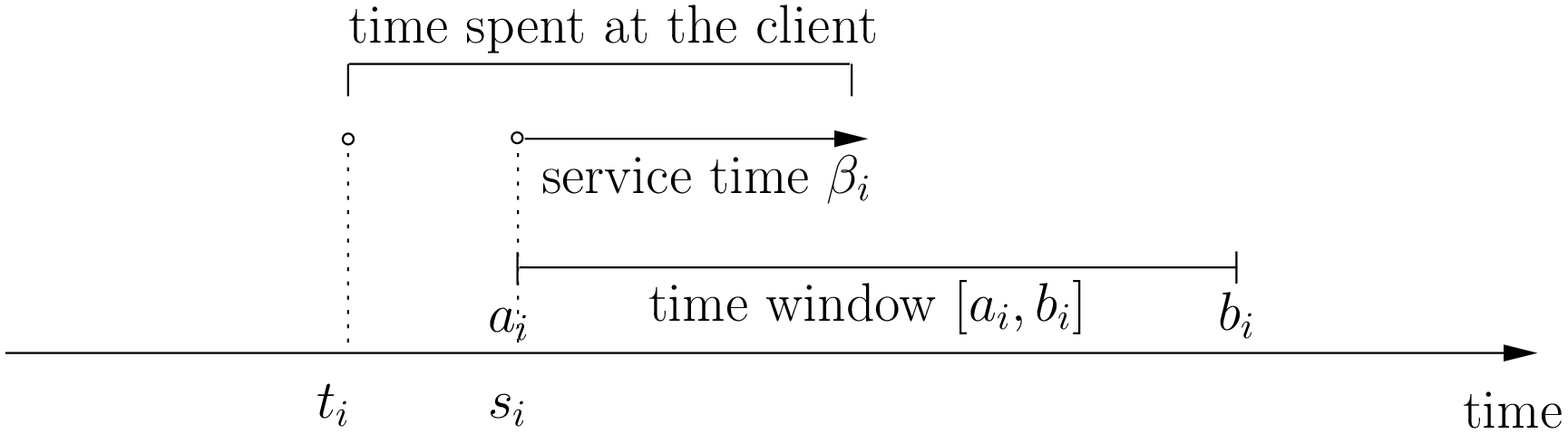
In real application, the time spent at a client might be limited to the service. For instance, you might wait in front
of the client’s office. It’s common to consider that you start to service and leave as soon as possible and
this is our assumption in this chapter
Some authors ([Dash2010] for instance) assign two costs on the edges: a travel cost and a travel time. While
the travel times must respect the time windows constraints, the objective value is the sum of the travel costs on the
edges. In this chapter, we only have one cost on the edges. The objective value and the real travel time are different: you might
have to wait before servicing a client.
| [Dash2010] | S. Dash, O. Günlük, A. Lodi, and A. Tramontani. A Time Bucket Formulation for the Traveling Salesman Problem with Time Windows, INFORMS Journal on Computing, v24, pp 132-147, 2012 (published online before print on December 29, 2010). |
Often, some conditions are applied to the time windows (in theory or practice). The only
condition[3] we will impose
is that  ,
,
i.e. we impose that the bounds of the time windows must be non negative integers. This also implies that the time windows
and the servicing times are finite.
| [3] | This condition doesn’t hold in Rodrigo Ferreira da Silva and Sebastián Urrutia’s definition of a TSPTW. In their article, they ask for (at least theoretically) 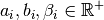 , i.e. non negative real numbers and , i.e. non negative real numbers and  . . |
The practical difficulty of the TSPTW is such that only instances with about 100 nodes have been solved to optimality[4] and heuristics rarely challenge instances with more than 400 nodes.
The
difficulty of the problem not only depends on the number of nodes but also on the “quality” of the time windows.
Not many attempts can be found in the scientific literature about exact or heuristic algorithms using CP to solve the TSPTW.
Actually, not so many attempts have been successful in solving this difficult problem in general.
The scientific literature on this problem is hence scarce.
We refer the interested reader to the two web pages cited in the next sub-section for some relevant literature.
9.8.2. Benchmark data
There isn’t a real standard. Basically, you’ll find two types of formats and their variants. We refer you
to two web pages because their respective authors took great care in formatting all the instances uniformly.
Manuel López-Ibáñez and Christian Blum have collected benchmark instances from different sources in
the literature. Their Benchmark Instances for the TSPTW page
contains about 300 instances.
Rodrigo Ferreira da Silva and Sebastián Urrutia also collected benchmark from different sources in the
literature. Their The TSPTW — Approaches & Additional Resources page
contains about 100 instances.
Both pages provide best solutions and sum up the relevant literature.
9.8.2.1. The López-Ibáñez-Blum format
We present the same instance proposed by Dumas et al. [Dumas1995] in both formats.
| [Dumas1995] | Dumas, Y., Desrosiers, J., Gelinas, E., Solomon, M., An optimal algorithm for the travelling salesman problem with time windows, Operations Research 43 (2) (1995) 367-371. |
Here is the content of the file n20w20.001.txt (LIB_n20w20.001.txt in our directory
/tutorials/cplusplus/chap9/):
21
0 19 17 34 7 20 10 17 28 15 23 29 23 29 21 20 9 16 21 13 12
19 0 10 41 26 3 27 25 15 17 17 14 18 48 17 6 21 14 17 13 31
17 10 0 47 23 13 26 15 25 22 26 24 27 44 7 5 23 21 25 18 29
34 41 47 0 36 39 25 51 36 24 27 38 25 44 54 45 25 28 26 28 27
7 26 23 36 0 27 11 17 35 22 30 36 30 22 25 26 14 23 28 20 10
20 3 13 39 27 0 26 27 12 15 14 11 15 49 20 9 20 11 14 11 30
10 27 26 25 11 26 0 26 31 14 23 32 22 25 31 28 6 17 21 15 4
17 25 15 51 17 27 26 0 39 31 38 38 38 34 13 20 26 31 36 28 27
28 15 25 36 35 12 31 39 0 17 9 2 11 56 32 21 24 13 11 15 35
15 17 22 24 22 15 14 31 17 0 9 18 8 39 29 21 8 4 7 4 18
23 17 26 27 30 14 23 38 9 9 0 11 2 48 33 23 17 7 2 10 27
29 14 24 38 36 11 32 38 2 18 11 0 13 57 31 20 25 14 13 17 36
23 18 27 25 30 15 22 38 11 8 2 13 0 47 34 24 16 7 2 10 26
29 48 44 44 22 49 25 34 56 39 48 57 47 0 46 48 31 42 46 40 21
21 17 7 54 25 20 31 13 32 29 33 31 34 46 0 11 29 28 32 25 33
20 6 5 45 26 9 28 20 21 21 23 20 24 48 11 0 23 19 22 17 32
9 21 23 25 14 20 6 26 24 8 17 25 16 31 29 23 0 11 15 9 10
16 14 21 28 23 11 17 31 13 4 7 14 7 42 28 19 11 0 5 3 21
21 17 25 26 28 14 21 36 11 7 2 13 2 46 32 22 15 5 0 8 25
13 13 18 28 20 11 15 28 15 4 10 17 10 40 25 17 9 3 8 0 19
12 31 29 27 10 30 4 27 35 18 27 36 26 21 33 32 10 21 25 19 0
0         408
62        68
181       205
306       324
214       217
51        61
102       129
175       186
250       263
3         23
21        49
79        90
78        96
140       154
354       386
42        63
2         13
24        42
20        33
9         21
275       300
The first line contains the number of nodes, including the depot. The n20w20.001 instance has a depot and 20 nodes.
The following 21 lines represent the distance matrix. This distance typically represents the
travel time between nodes and  , plus the service time at node .
The distance matrix is not necessarily symmetrical. The last 21 lines represent the time windows (earliest, latest)
for each node, one per line. The first node is the depot.
When then sum of service times is not 0, it is specified in a comment on the last line:
# Sum of service times: 522
9.8.2.2. The da Silva-Urrutia format
We present exactly the same instance as above. Here is the file n20w20.001.txt (DSU_n20w20.001.txt
in our directory /tutorials/cplusplus/chap9/):
!! n20w20.001    16.75 391

CUST NO. XCOORD. YCOORD. DEMAND [READY TIME] [DUE DATE] [SERVICE TIME]

    1    16.00    23.00   0.00      0.00       408.00       0.00
    2    22.00     4.00   0.00     62.00        68.00       0.00
    3    12.00     6.00   0.00    181.00       205.00       0.00
    4    47.00    38.00   0.00    306.00       324.00       0.00
    5    11.00    29.00   0.00    214.00       217.00       0.00
    6    25.00     5.00   0.00     51.00        61.00       0.00
    7    22.00    31.00   0.00    102.00       129.00       0.00
    8     0.00    16.00   0.00    175.00       186.00       0.00
    9    37.00     3.00   0.00    250.00       263.00       0.00
   10    31.00    19.00   0.00      3.00        23.00       0.00
   11    38.00    12.00   0.00     21.00        49.00       0.00
   12    36.00     1.00   0.00     79.00        90.00       0.00
   13    38.00    14.00   0.00     78.00        96.00       0.00
   14     4.00    50.00   0.00    140.00       154.00       0.00
   15     5.00     4.00   0.00    354.00       386.00       0.00
   16    16.00     3.00   0.00     42.00        63.00       0.00
   17    25.00    25.00   0.00      2.00        13.00       0.00
   18    31.00    15.00   0.00     24.00        42.00       0.00
   19    36.00    14.00   0.00     20.00        33.00       0.00
   20    28.00    16.00   0.00      9.00        21.00       0.00
   21    20.00    35.00   0.00    275.00       300.00       0.00
  999     0.00     0.00   0.00      0.00         0.00       0.00
Having seen the same instance, you don’t need much complementary info to
understand this format. The first line of data (CUST NO. 1) represents the depot and
the last line marks the end of the file. As you can see, the authors are not really optimistic about solving
instances with more than 999 nodes! We don’t use the DEMAND column and we round down the numbers of the last three
columns.
You might think that the translation from this second
format to the first one is obvious. It is not! See the
remark on Travel-time Computation on the
Jeffrey Ohlmann and Barrett Thomas benchmark page.
In the code, we don’t try to match the data between the two formats, so you might encounter different solutions.
Warning
The same instances in the da Silva-Urrutia and the López-Ibáñez-Blum formats might be slightly different.
9.8.2.3. Solutions
We use a simple format to record feasible solutions:
- a first line with a permutation of the nodes;
- a second line with the objective value.
For our instance, here is an example of a feasible solution:
1 17 10 20 18 19 11 6 16 2 12 13 7 14 8 3 5 9 21 4 15
378
The objective value 378 is the sum of the costs of the arcs and not the time spent to travel (which is 387
in this case).
A basic program check_tsptw_solutions.cc verifies if a given solution is indeed feasible for a given instance
in López-Ibáñez-Blum or da Silva-Urrutia formats:
./check_tsptw_solutions -tsptw_data_file=DSU_n20w20.001.txt
                                 -tsptw_solution_file=n20w20.001.sol
This program checks if all the nodes have been serviced and if the solution is feasible:
bool IsFeasibleSolution() {
  ...
  //  for loop to test each node in the tour
  for (...) {
    //  Test if we have to wait at client node
    waiting_time = ReadyTime(node) - total_time;
    if (waiting_time > 0) {
      total_time = ReadyTime(node);
    }
    if (total_time + ServiceTime(node) > DueTime(node)) {
      return false;
    }
  }
  ...
  return true;
}
IsFeasibleSolution() returns true if the submitted solution is feasible and false otherwise. To test this
solution, we construct the tour node by node. Arriving at a node node at time total_time
in the for loop, we test two things:
-
First, if we have to wait. We compute the waiting time waiting_time: ReadyTime(node) returns
the ready time of the node node
and total_time is the total time spent in the tour to reach the node node. If the ready time is greater than
total_time, waiting_time > 0 is true and we set total_time to ReadyTime(node). -
Second, if the due times are respected, i.e.:
is total_time + ServiceTime(node)
 DueTime(node) true?
If not, the method returns false. If all the due times are respected, the method returns true.

The output of the above command line is:
TSPTW instance of type da Silva-Urrutia format
Solution is feasible!
Loaded obj value: 378, Computed obj value: 387
Total computed travel time: 391
TSPTW file DSU_n20w20.001.txt (n=21, min=2, max=59, sym? yes)
(!! n20w20.001 16.75 391 )
As you can see, the recorded objective value in the solution file is 378 while the value of the computed
objective value is 387. This is because the distance matrix computed is different from the actual one
really used
to compute the objective value of the solution. We refer again the reader to the remark on Travel-time Computation
from Jeffrey Ohlmann and Barrett Thomas cited above. If you use the right distance matrix as in the
López-Ibáñez-Blum format, you get:
TSPTW instance of type López-Ibáñez-Blum format
Solution is feasible!
Loaded obj value: 378, Computed obj value: 378
Total computed travel time: 387
TSPTW file LIB_n20w20.001.txt (n=21, min=2, max=57, sym? yes)
Now both the given objective value and the computed one are equal. Note that the total travel time is a bit longer:
387 for a total distance of 378.
9.8.3. The TSPTWData class
You’ll find the code in the file tsptw.h.
The TSPTWData class is modelled on the TSPData class. As in the case of the TSPLIB,
we number the nodes starting from one.
9.8.3.1. To read instance files
To read TSPTW instance files, the TSPTWData class offers the
LoadTSPTWFile(const std::string& filename);
method.
It parses a file in López-Ibáñez-Blum or da Silva-Urrutia format and — in the second case — loads the coordinates
and the service times for further treatment. Note that the instance’s format is only partially checked: bad inputs might cause
undefined behaviour.
To test if the instance was successfully loaded, use:
bool IsInstanceLoaded() const;
Several specialized getters are available:
- std::string Name() const: returns the instance name, here the filename of the instance;
- std::string InstanceDetails() const: returns a short description of the instance;
- int Size() const: returns the size of the instance;
- int64 Horizon() const: returns the horizon of the instance, i.e. the maximal due time;
- int64 Distance(RoutingModel::NodeIndex from, RoutingModel::NodeIndex to) const: returns the distance between the
two NodeIndexes; - RoutingModel::NodeIndex Depot() const: returns the depot. This the first node given in the instance and solutions
files. - int64 ReadyTime(RoutingModel::NodeIndex i) const: returns the ready time of node i;
- int64 DueTime(RoutingModel::NodeIndex i) const: returns the due time of node i
- int64 ServiceTime(RoutingModel::NodeIndex i) const: returns the service time of node i.
The ServiceTime() method only makes sense when an instance is given in the da Silva-Urrutia format. In the
López-Ibáñez-Blum format, the service times are added to the arc costs in the “distance” matrix
and the ServiceTime() method returns 0.
To model the time windows in the RT, we use Dimensions, i.e. quantities that are accumulated along the routes at each
node.
At a given node to, the accumulated time is the travel cost of the arc (from, to) plus the time to service
the node to. The TSPTWData class has a special
method to return this quantity:
int64 CumulTime(RoutingModel::NodeIndex from,
                RoutingModel::NodeIndex to) const {
  return Distance(from, to) + ServiceTime(from);
}
9.8.3.2. To read solution files
To read solution files, use the
void LoadTSPTWSolutionFile(const std::string& filename);
method. This way, you can
load solution files and test them with the bool IsFeasibleSolution() method briefly seen above.
Actually, you should enquire if the solution is feasible before doing anything with it.
Three methods help you deal with the existence/feasibility of the solution:
bool IsSolutionLoaded() const;
bool IsSolution() const;
bool IsFeasibleSolution() const;
With IsSolutionLoaded() you can check that indeed a solution was loaded/read from a file. IsSolution() tests
if the solution contains once and only once all the nodes of the graph while IsFeasibleSolution() tests if
the loaded solution
is feasible, i.e. if all due times are respected.
Once you are sure that a solution is valid and feasible, you can query the loaded solution:
- int64 SolutionComputedTotalTravelTime() const: computes the total travel time and returns it. The travel total time
often differs from the objective value because of waiting times; - int64 SolutionComputedObjective() const: computes the objective value and returns it;
- int64 SolutionLoadedObjective() const: returns the objective value stored in the instance file
These methods are also available if the solution was obtained by the solver (in this case, SolutionLoadedObjective()
returns -1 and IsSolutionLoaded() returns false).
The TSPTWData class doesn’t generate random instances. We wrote a little program for this purpose.
9.8.4. Random generation of instances
You’ll find the code in the file tsptw_generator.cc.
The TSPTW instance generator tsptw_generator is very basic. It generates an instance in
López-Ibáñez-Blum or/and da Silva-Urrutia as follows:
- it generates random points in the plane;
- it generates a random tour;
- it generates random service times and
- it generates random time windows such that the random solution is feasible.
 random points in the plane;
Several parameters (gflags) are defined to control the output:
- tsptw_name: The name of the instance;
- tsptw_size: The number of clients including the depot;
- tsptw_deterministic_random_seed: Use deterministic random seeds or not? (default: true);
- tsptw_time_window_min: Minimum window time length (default: 10);
- tsptw_time_window_max: Maximum window time length (default: 30);
- tsptw_service_time_min: Minimum service time length (default: 0);
- tsptw_service_time_max: Maximum service time length (default: 10);
- tsptw_x_max: Maximum x coordinate (default: 100);
- tsptw_y_max: Maximum y coordinate (default: 100);
- tsptw_LIB: Create a López-Ibáñez-Blum format instance file or not? (default: true);
- tsptw_DSU: Create a da Silva-Urrutia format instance file or not? (default: true);
By default, if the name of the instance is
myInstance, tsptw_generator creates the three files:
- DSU_myInstance.txt;
- LIB_myInstance.txt and
- myInstance_init.sol.
myInstance_init.sol contains the random tour generated to create the instance. Files with the same name are
overwritten without mercy.
9.8.5. Visualization with ePix
To visualize the solutions, we rely again on the
excellent ePiX library. The
file tsptw_epix.h contains the TSPTWEpixData class. This class is similar to the TSPEpixData class.
Its unique constructor reads:
RoutingModel routing(...);
...
TSPTWData data(...);
...
TSPTWEpixData(const RoutingModel& routing,
              const TSPTWData& data);
To write a ePiX solution file, use the following methods:
void WriteSolutionFile(const Assignment * solution,
                       const std::string & epix_filename)
void WriteSolutionFile(const std::string & tpstw_solution_filename,
                       const std::string & epix_filename);
The first method takes an Assignment while the second method reads the solution from a solution file.
You can define the width and height of the generated image:
DEFINE_int32(epix_width, 10, "Width of the pictures in cm.");
DEFINE_int32(epix_height, 10, "Height  of the pictures in cm.");
Once the ePiX file is written, you must evoke the ePiX elaps script:
./elaps -pdf epix_file.xp
Here is an example of the solution in the file n20w20.001.sol:
The dot in red in the center represents the depot or first node. The arrows indicate the direction of the tour. Because of the time
windows, the solution is no longer planar, i.e. the tour crosses itself.
You can also print the node labels and the time windows with the flags:
DEFINE_bool(tsptw_epix_labels, false, "Print labels or not?");
DEFINE_bool(tsptw_epix_time_windows, false,
                                      "Print time windows or not?");
For your (and our!) convenience, we wrote a small program tsptw_solution_to_epix.
Its implementation is in the file tsptw_solution_to_epix.cc. To use it, invoke:
./tsptw_solution_to_epix TSPTW_instance_file TSPTW_solution_file >
                                                epix_file.xp
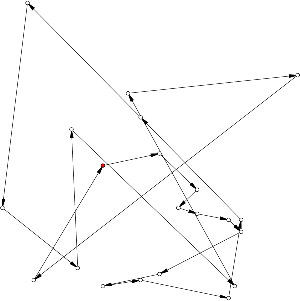
I’m trying to solve TSP problem with additional constraint — time windows.
All the standard assumptions apply:
- We start and end at given city.
- Each city is visited only once.
- We try to find the optimal path in terms of travel cost (here travel time).
Additionally each city has its own time window in format , which limits when a city can be visited:
- We cannot visit a city after its closing time.
- We can arrive at any city before it’s opening time and wait for it to open. If we do so, waiting time is added to overall time passed, but it is not added to time spent travelling. So time_spent_travelling and total_time_passed are two distinct things we need to keep track of.
I managed to write constraints that find optimal solution in terms of total_time_passed, but I need to find optimal time_spent_travelling.
Here is my logic:
% THE TRAVELING SALESMAN WITH TIME WINDOWS

% DESC ------------------------------------------------------------------------------------
% visited(city, arrive_step)
% travel(dest_city, depart_step)
% location(city, arrive_step, when_visited (summary travel time))
% place(name, opening_time, closing_time)
% path(from, to, travel_cost)

% Warunki ----------------------------------------------------------------------------------

% Start and end must be in the same city
:- not location(Place, t, _), location(Place, 0, _).

% Paths are symmetrical
path(A, B, COST) :- path(B, A, COST).

% In each step, there can be only one travel from one city to another
{ travel(Place, T) : place(Place, _, _) } 1 :- T = 0..t-1.

% If there was a travel to a city, that city has been visited (this way starting city is not visited at the beginning)
visited(Place, T) :- travel(Place, T).

% We cannot visit a city, we've been to before
:- travel(Place, T1), visited(Place, T2), T1 > T2.

% We cannot travel to city, we are staying right now
:- travel(Place, T), location(Place, T, _).

% We cannot go to somewhere, to where leads no path
:- travel(To, T), location(From, T, _), not path(From, To, _).

% We cannot travel to city if we arrive after it's closing time
:- travel(TO, T), location(From, T, TOTAL_TIME), path(From, TO, TRAVEL_TIME), place(TO, OPENED_FROM, OPENED_TO), TOTAL_TIME + TRAVEL_TIME > OPENED_TO.

% If we started travel to city A at step T, we must have reached it at step T + 1
% City might me not opened yet, so our travel time is MAX of (CITY_OPENED_TIME, ARRIVAL_TIME)
% max = ((a+b)+|a-b|)/2
% min = ((a+b)-|a-b|)/2
location(To, T + 1, ((ARRIVAL+OPENED_FROM)+|ARRIVAL-OPENED_FROM|)/2) :-  travel(To, T), location(From, T, C1) , path(From, To, C2), place(To, OPENED_FROM, _), ARRIVAL = C1+C2.

% There isn't a single city, we haven't visited
:- place(Place, _, _), not visited(Place, _).

% Find minimal travel time (Arrival time at starting city)
result(C) :- location(_, t, C).
#minimize{C : result(C)}.

#show location/3.
And here sample data (Running it with clingo takes ~ 30s):
% Cities count
#const t=21.

% Starting point
location(city_0, 0, 0).

% City list in format (name, opening_time, closing_time)
place(city_0, 0, 408).
place(city_1, 62, 68).
place(city_2, 181, 205).
place(city_3, 306, 324).
place(city_4, 214, 217).
place(city_5, 51, 61).
place(city_6, 102, 129).
place(city_7, 175, 186).
place(city_8, 250, 263).
place(city_9, 3, 23).
place(city_10, 21, 49).
place(city_11, 79, 90).
place(city_12, 78, 96).
place(city_13, 140, 154).
place(city_14, 354, 386).
place(city_15, 42, 63).
place(city_16, 2, 13).
place(city_17, 24, 42).
place(city_18, 20, 33).
place(city_19, 9, 21).
place(city_20, 275, 300).

% Distance between cities (from, to, travel_cost)
path(city_0, city_1, 19).
path(city_0, city_2, 17).
path(city_0, city_3, 34).
path(city_0, city_4, 7).
path(city_0, city_5, 20).
path(city_0, city_6, 10).
path(city_0, city_7, 17).
path(city_0, city_8, 28).
path(city_0, city_9, 15).
path(city_0, city_10, 23).
path(city_0, city_11, 29).
path(city_0, city_12, 23).
path(city_0, city_13, 29).
path(city_0, city_14, 21).
path(city_0, city_15, 20).
path(city_0, city_16, 9).
path(city_0, city_17, 16).
path(city_0, city_18, 21).
path(city_0, city_19, 13).
path(city_0, city_20, 12).
path(city_1, city_2, 10).
path(city_1, city_3, 41).
path(city_1, city_4, 26).
path(city_1, city_5, 3).
path(city_1, city_6, 27).
path(city_1, city_7, 25).
path(city_1, city_8, 15).
path(city_1, city_9, 17).
path(city_1, city_10, 17).
path(city_1, city_11, 14).
path(city_1, city_12, 18).
path(city_1, city_13, 48).
path(city_1, city_14, 17).
path(city_1, city_15, 6).
path(city_1, city_16, 21).
path(city_1, city_17, 14).
path(city_1, city_18, 17).
path(city_1, city_19, 13).
path(city_1, city_20, 31).
path(city_2, city_3, 47).
path(city_2, city_4, 23).
path(city_2, city_5, 13).
path(city_2, city_6, 26).
path(city_2, city_7, 15).
path(city_2, city_8, 25).
path(city_2, city_9, 22).
path(city_2, city_10, 26).
path(city_2, city_11, 24).
path(city_2, city_12, 27).
path(city_2, city_13, 44).
path(city_2, city_14, 7).
path(city_2, city_15, 5).
path(city_2, city_16, 23).
path(city_2, city_17, 21).
path(city_2, city_18, 25).
path(city_2, city_19, 18).
path(city_2, city_20, 29).
path(city_3, city_4, 36).
path(city_3, city_5, 39).
path(city_3, city_6, 25).
path(city_3, city_7, 51).
path(city_3, city_8, 36).
path(city_3, city_9, 24).
path(city_3, city_10, 27).
path(city_3, city_11, 38).
path(city_3, city_12, 25).
path(city_3, city_13, 44).
path(city_3, city_14, 54).
path(city_3, city_15, 45).
path(city_3, city_16, 25).
path(city_3, city_17, 28).
path(city_3, city_18, 26).
path(city_3, city_19, 28).
path(city_3, city_20, 27).
path(city_4, city_5, 27).
path(city_4, city_6, 11).
path(city_4, city_7, 17).
path(city_4, city_8, 35).
path(city_4, city_9, 22).
path(city_4, city_10, 30).
path(city_4, city_11, 36).
path(city_4, city_12, 30).
path(city_4, city_13, 22).
path(city_4, city_14, 25).
path(city_4, city_15, 26).
path(city_4, city_16, 14).
path(city_4, city_17, 23).
path(city_4, city_18, 28).
path(city_4, city_19, 20).
path(city_4, city_20, 10).
path(city_5, city_6, 26).
path(city_5, city_7, 27).
path(city_5, city_8, 12).
path(city_5, city_9, 15).
path(city_5, city_10, 14).
path(city_5, city_11, 11).
path(city_5, city_12, 15).
path(city_5, city_13, 49).
path(city_5, city_14, 20).
path(city_5, city_15, 9).
path(city_5, city_16, 20).
path(city_5, city_17, 11).
path(city_5, city_18, 14).
path(city_5, city_19, 11).
path(city_5, city_20, 30).
path(city_6, city_7, 26).
path(city_6, city_8, 31).
path(city_6, city_9, 14).
path(city_6, city_10, 23).
path(city_6, city_11, 32).
path(city_6, city_12, 22).
path(city_6, city_13, 25).
path(city_6, city_14, 31).
path(city_6, city_15, 28).
path(city_6, city_16, 6).
path(city_6, city_17, 17).
path(city_6, city_18, 21).
path(city_6, city_19, 15).
path(city_6, city_20, 4).
path(city_7, city_8, 39).
path(city_7, city_9, 31).
path(city_7, city_10, 38).
path(city_7, city_11, 38).
path(city_7, city_12, 38).
path(city_7, city_13, 34).
path(city_7, city_14, 13).
path(city_7, city_15, 20).
path(city_7, city_16, 26).
path(city_7, city_17, 31).
path(city_7, city_18, 36).
path(city_7, city_19, 28).
path(city_7, city_20, 27).
path(city_8, city_9, 17).
path(city_8, city_10, 9).
path(city_8, city_11, 2).
path(city_8, city_12, 11).
path(city_8, city_13, 56).
path(city_8, city_14, 32).
path(city_8, city_15, 21).
path(city_8, city_16, 24).
path(city_8, city_17, 13).
path(city_8, city_18, 11).
path(city_8, city_19, 15).
path(city_8, city_20, 35).
path(city_9, city_10, 9).
path(city_9, city_11, 18).
path(city_9, city_12, 8).
path(city_9, city_13, 39).
path(city_9, city_14, 29).
path(city_9, city_15, 21).
path(city_9, city_16, 8).
path(city_9, city_17, 4).
path(city_9, city_18, 7).
path(city_9, city_19, 4).
path(city_9, city_20, 18).
path(city_10, city_11, 11).
path(city_10, city_12, 2).
path(city_10, city_13, 48).
path(city_10, city_14, 33).
path(city_10, city_15, 23).
path(city_10, city_16, 17).
path(city_10, city_17, 7).
path(city_10, city_18, 2).
path(city_10, city_19, 10).
path(city_10, city_20, 27).
path(city_11, city_12, 13).
path(city_11, city_13, 57).
path(city_11, city_14, 31).
path(city_11, city_15, 20).
path(city_11, city_16, 25).
path(city_11, city_17, 14).
path(city_11, city_18, 13).
path(city_11, city_19, 17).
path(city_11, city_20, 36).
path(city_12, city_13, 47).
path(city_12, city_14, 34).
path(city_12, city_15, 24).
path(city_12, city_16, 16).
path(city_12, city_17, 7).
path(city_12, city_18, 2).
path(city_12, city_19, 10).
path(city_12, city_20, 26).
path(city_13, city_14, 46).
path(city_13, city_15, 48).
path(city_13, city_16, 31).
path(city_13, city_17, 42).
path(city_13, city_18, 46).
path(city_13, city_19, 40).
path(city_13, city_20, 21).
path(city_14, city_15, 11).
path(city_14, city_16, 29).
path(city_14, city_17, 28).
path(city_14, city_18, 32).
path(city_14, city_19, 25).
path(city_14, city_20, 33).
path(city_15, city_16, 23).
path(city_15, city_17, 19).
path(city_15, city_18, 22).
path(city_15, city_19, 17).
path(city_15, city_20, 32).
path(city_16, city_17, 11).
path(city_16, city_18, 15).
path(city_16, city_19, 9).
path(city_16, city_20, 10).
path(city_17, city_18, 5).
path(city_17, city_19, 3).
path(city_17, city_20, 21).
path(city_18, city_19, 8).
path(city_18, city_20, 25).
path(city_19, city_20, 19).
I used MAX function to calculate arrival time at given cities by choosing from real arrival time or city’s opening time — whichever happened to be later. It worked nicely, so my first thought was to add additional field to location fact changing this line as follows:
%Before:
location(To, T + 1, ((ARRIVAL+OPENED_FROM)+|ARRIVAL-OPENED_FROM|)/2) :-  travel(To, T), location(From, T, C1) , path(From, To, C2), place(To, OPENED_FROM, _), ARRIVAL = C1+C2.
%After:
location(To, T + 1, ((ARRIVAL+OPENED_FROM)+|ARRIVAL-OPENED_FROM|)/2, TRAVEL_TIME + C2) :-  travel(To, T), location(From, T, C1, TRAVEL_TIME) , path(From, To, C2), place(To, OPENED_FROM, _), ARRIVAL = C1+C2.
This way location hold information about both time_spent_travelling and total_time_passed. While this works fine for 5 cities, with 20 cities it keeps calculating too long (I gave up after 15 minutes) — I expected the program to run roughly the same time at both situations, but apparently there is something I don’t understand here.
I also tried to store waiting times as separate facts, but it seemed to affect computing time the same way and introduced another issue of taking it into consideration in #minimize function which I couldn’t menage to solve.
So here are my questions:
- What can I do to calculate optimal value of time_spent_travelling, yet correctly considering waiting time?
- Why a small change in code, I’ve described above, has such a high computational impact on the solving process?
I’ve started using clingo recently and there is a good chance I don’t see a simple solution to this problem. It’s kind of hard to change the way you write your program, being so used to declarative programming.
The code I’ve provided can be simple run with clingo:
clingo logic data
My output:
Solving...
Answer: 1
location(city_0,0,0) location(city_16,1,9) location(city_9,2,17) location(city_19,3,21) location(city_17,4,24) location(city_10,5,31) location(city_18,6,33) location(city_5,7,51) location(city_15,8,60) location(city_1,9,66) location(city_11,10,80) location(city_12,11,93) location(city_6,12,115) location(city_13,13,140) location(city_7,14,175) location(city_2,15,190) location(city_4,16,214) location(city_8,17,250) location(city_20,18,285) location(city_3,19,312) location(city_14,20,366) location(city_0,21,387)
Optimization: 387
OPTIMUM FOUND

Models       : 1
  Optimum    : yes
Optimization : 387
Calls        : 1
Time         : 27.654s (Solving: 0.10s 1st Model: 0.04s Unsat: 0.06s)
CPU Time     : 27.651s
(base) igor@i:~/projects/transInfo/TSPTW/src$ clingo dane logika
clingo version 5.4.0
Reading from dane ...
Solving...
Answer: 1
location(city_0,0,0) location(city_16,1,9) location(city_9,2,17) location(city_19,3,21) location(city_17,4,24) location(city_10,5,31) location(city_18,6,33) location(city_5,7,51) location(city_15,8,60) location(city_1,9,66) location(city_11,10,80) location(city_12,11,93) location(city_6,12,115) location(city_13,13,140) location(city_7,14,175) location(city_2,15,190) location(city_4,16,214) location(city_8,17,250) location(city_20,18,285) location(city_3,19,312) location(city_14,20,366) location(city_0,21,387)
Optimization: 387
OPTIMUM FOUND

Models       : 1
  Optimum    : yes
Optimization : 387
Calls        : 1
Time         : 29.682s (Solving: 0.09s 1st Model: 0.03s Unsat: 0.06s)
CPU Time     : 29.680s
Here the result takes into consideration waiting time, which in this particular example is 9. (378 is time spent only on travelling).
Содержание
- Travelling Salesman Problem with Time Windows
- I’m trying to solve TSP problem with additional constraint — time windows.
- So here are my questions:
- Multiple Traveling Salesman Problem (mTSP)
- Case Study Contents
- Problem Statement
- Mathematical Formulation
- GAMS Model
- Multiple traveling salesman problem with time windows
Travelling Salesman Problem with Time Windows
I’m trying to solve TSP problem with additional constraint — time windows.
All the standard assumptions apply:
- We start and end at given city.
- Each city is visited only once.
- We try to find the optimal path in terms of travel cost (here travel time).
Additionally each city has its own time window in format , which limits when a city can be visited:
- We cannot visit a city after its closing time.
- We can arrive at any city before it’s opening time and wait for it to open. If we do so, waiting time is added to overall time passed, but it is not added to time spent travelling. So time_spent_travelling and total_time_passed are two distinct things we need to keep track of.
I managed to write constraints that find optimal solution in terms of total_time_passed, but I need to find optimal time_spent_travelling.
Here is my logic:
And here sample data (Running it with clingo takes
I used MAX function to calculate arrival time at given cities by choosing from real arrival time or city’s opening time — whichever happened to be later. It worked nicely, so my first thought was to add additional field to location fact changing this line as follows:
This way location hold information about both time_spent_travelling and total_time_passed. While this works fine for 5 cities, with 20 cities it keeps calculating too long (I gave up after 15 minutes) — I expected the program to run roughly the same time at both situations, but apparently there is something I don’t understand here.
I also tried to store waiting times as separate facts, but it seemed to affect computing time the same way and introduced another issue of taking it into consideration in #minimize function which I couldn’t menage to solve.
So here are my questions:
- What can I do to calculate optimal value of time_spent_travelling, yet correctly considering waiting time?
- Why a small change in code, I’ve described above, has such a high computational impact on the solving process?
I’ve started using clingo recently and there is a good chance I don’t see a simple solution to this problem. It’s kind of hard to change the way you write your program, being so used to declarative programming.
The code I’ve provided can be simple run with clingo: clingo logic data
Here the result takes into consideration waiting time, which in this particular example is 9. (378 is time spent only on travelling).
Multiple Traveling Salesman Problem (mTSP)
Summary: The Multiple Traveling Salesman Problem ((m)TSP) is a generalization of the Traveling Salesman Problem (TSP) in which more than one salesman is allowed. Given a set of cities, one depot where (m) salesmen are located, and a cost metric, the objective of the (m)TSP is to determine a tour for each salesman such that the total tour cost is minimized and that each city is visited exactly once by only one salesman.
Case Study Contents
Problem Statement
The Multiple Traveling Salesman Problem ((m)TSP) is a generalization of the Traveling Salesman Problem (TSP) in which more than one salesman is allowed. Given a set of cities, one depot (where (m) salesmen are located), and a cost metric, the objective of the (m)TSP is to determine a set of routes for (m) salesmen so as to minimize the total cost of the (m) routes. The cost metric can represent cost, distance, or time. The requirements on the set of routes are:
- All of the routes must start and end at the (same) depot.
- Each city must be visited exactly once by only one salesman.
The (m)TSP is a relaxation of the vehicle routing problem (VRP); if the vehicle capacity in the VRP is a sufficiently large value so as not to restrict the vehicle capacity, then the problem is the same as the (m)TSP. Therefore, all of the formulations and solution approaches for the VRP are valid for the (m)TSP. The (m)TSP is a generalization of the TSP; if the value of (m) is 1, then the (m)TSP problem is the same as the TSP. Therefore, all of the formulations and solution approaches for the (m)TSP are valid for the TSP.
Bektas (2006) lists a number of variations on the (m)TSP.
- Multiple depots: Instead of one depot, the multi-depot (m)TSP has a set of depots, with (m_j) salesmen at each depot (j). In the fixed destination version, a salesman returns to the same depot from which he started. In the non-fixed destination version, a salesman does not need to return to the same depot from which he started but the same number of salesmen must return as started from a particular depot. The multi-depot (m)TSP is important in robotic applications involving ground and aerial vehicles. For example, see Oberlin et al. (2009).
- Specifications on the number of salesmen: The number of salesmen may be a fixed number (m), or the number of salesmen may be determined by the solution but bounded by an upper bound (m).
- Fixed charges: When the number of salesmen is not fixed, there may be a fixed cost associated with activating a salesman. In the fixed charge version of the (m)TSP, the overall cost to minimize includes the fixed charges for the salesmen plus the costs for the tours.
- Time windows: As with the TSP and the VRP, there is a variation of the (m)TSP with time windows. Associated with each node is a time window during which the node must be visited by a tour. The (m)TSPTW has many applications, such as school bus routing and airline scheduling.
Mathematical Formulation
Here we present an assignment-based integer programming formulation for the (m)TSP.
Consider a graph (G=(V,A)), where (V) is the set of (n) nodes, and (A) is the set of edges. Associated with each edge ((i,j) in A) is a cost (or distance) (c_). We assume that the depot is node 1 and there are (m) salesmen at the depot. We define a binary variable (x_) for each edge ((i,j) in A); (x_) takes the value 1 if edge ((i,j)) is included in a tour and (x_) takes the value 0 otherwise. For the subtour elimination constraints, we define an integer variable (u_i) to denote the position of node (i) in a tour, and we define a value (p) to be the maximum number of nodes that can be visited by any salesman.
Constraints
Ensure that exactly (m) salesmen depart from node 1
(sum_ x_ <1j>= m)
Ensure that exactly (m) salesmen return to node 1
(sum_ x_ = m)
Ensure that exactly one tour enters each node
(sum_ x_ = 1, forall j in V)
Ensure that exactly one tour exits each node
(sum_ x_ = 1, forall i in V)
Include subtour elimination constraints (Miller-Tucker-Zemlin)
(u_i — u_j + p cdot x_ leq p-1, forall 2 leq i neq j leq n)
The literature includes a number of alternative formulations. Some of the alternatives to the two-index variable, assignment-based formulation are a two-index variable formulation with the original subtour elimination constraints (see Laporte and Nobert, 1980), a three-index variable formulation (see Bektas, 2006), and a (k)-degree center tree-based formulation (see Christofides et al., 1981 and Laporte, 1992).
To solve this integer linear programming problem, we can use one of the NEOS Server solvers in the Mixed Integer Linear Programming (MILP) category. Each MILP solver has one or more input formats that it accepts.
GAMS Model
Click here for a GAMS model for the bayg29 instance from the TSPLIB. The formulation was provided by Erwin Kalvelagen in a blog post here.
If we submit this model to XpressMP with a CPU time limit of 1 hour, we obtain a solution with a total cost of 2176 (gap of 4.3%) and the following tours:
- Tour 1: i13 — i4 — i10 — i20 — i2 — i13
cost = 60 + 39 + 25 + 49 + 87 = 260 - Tour 2: i13 — i18 — i14 — i17 — i22 — i11 — i15 — i13
cost = 128 + 32 + 51 + 47 + 63 + 68 + 86 = 475 - Tour 3: i13 — i24 — i8 — i28 — i12 — i6 — i1 — i13
cost = 56 + 48 + 64 + 71 + 46 + 60 + 82 = 427 - Tour 4: i13 — i29 — i3 — i26 — i9 — i5 — i21 — i13
cost =160 + 60 + 78 + 57 + 42 + 50 + 82 = 529 - Tour 5: i13 — i19 — i25 — i7 — i23 — i27 — i16 — i13
cost = 71 + 52 + 72 + 111 + 74 + 48 + 57 = 485
Multiple traveling salesman problem with time windows
The Multiple Traveling Salesman Problem
The Multiple Traveling Salesman Problem (mTSP) in which more than one salesman is allowed is a generalization of the Traveling Salesman Problem (TSP). Given a set of cities, one depot (where m salesmen are located), and a cost metric, the objective of the mTSP is to determine a set of routes for m salesmen so as to minimize the total cost of the m routes. The cost metric can represent cost, distance, or time. The requirements on the set of routes are:
- All of the routes must start and end at the (same) depot.
- There must be at least one city (except depot) in each route.
- Each city must be visited exactly once by only one salesman.
Multiple depots: Instead of one depot, the multi-depot mTSP has a set of depots, with mj salesmen at each depot j. In the fixed destination version, a salesman returns to the same depot from which he started.
Please keep in mind that this project is based on the 81 cities of Turkey while examining sample solutions given below.
In this part of the homework, we will generate 100,000 random solutions to the fixed destination version of the multi-depot mTSP. The number of depots and salesman per depot will be our parameters. The cost metric will be total distance in kilometers. At the end, we will print the best solution that has the minimum cost among 100,000 random solutions.
Your project must be a valid maven project. mvn clean package must produce an executable jar file named mTSP.jar under the target directory. This can be done via maven plugins such as shade or assembly plugin. Optional parameter finalName can be used to change the name of the shaded artifactId. To parse command line arguments, you must use JewelCLI library.
For example, java -jar target/mTSP.jar -d 5 -s 2 -v would produce something like below. Notice that the last line includes the cost metric: the total distance travelled by all salesmen.
Non-verbose example java -jar target/mTSP.jar -d 2 -s 5 will print city indices instead of city names:
❗ If you don’t follow the aforementioned conventions, you will receive grade of zero (even if you think that your code works perfectly).
In the second part of the homework, we will apply a heuristic algorithm to our fixed destination version of the multi-depot mTSP.
The term heuristic is used for algorithms which find solutions among all possible ones, but they do not guarantee that the optimal will be found. Heuristic algorithms often times used to solve NP-complete problems.
The heuristic will iteratively work on the solution (best of the 100,000 random solutions) obtained from the Part-I. In Part-II, we will define five different move operations, which will be detailed in the following subsections. In each iteration, one move operation will be selected (among five) based on a random manner, and then it will be applied to the current solution. If the move improves the solution (i.e., lessen the total distance travelled) then, we will update the best solution at hand. If not, next iteration will be continued. To implement this logic, you need to devise a strategy to somehow backup the current solution. So that if the subsequent move operation does not improve the solution, it should be possible to rollback to a previous state. It is recommended to do a reach on the Internet using the following keywords: copy constructor, deep cloning, shallow cloning, and marshalling. It is totally up to you to how to implement this logic, you can even write an method that calculates a cost function without applying the move!
Some of the the move operation will involve a process where you need to generate two different random numbers from a given interval. Please write a method to generate two random numbers that are different from each other. Here comes the five move operations that the heuristic will be using.
Swap two nodes in a route. Here, both the route and the two nodes are randomly chosen. In this move we select a random route among all routes and then we swap two nodes. Remember to avoid no-operation, we need to select two nodes that are different from each other. Example of the move: random node indices are 1 and 7, which are shown in bold.
Notice that bold nodes are swapped with each other after the move.
Swap hub with a randomly chosen node in a route. Here, both the route and the node are randomly chosen. In this move we select a random route among all routes and then we replace the hub with a random node. Here it is crucial to update the hub in the remaining routes of the initial hub.
Example of the move: random node index is 10, which is shown in bold.
Notice that bold node is replaced with the hub in the first route. Notice also that hub of the second route is updated. Nodes of the second route remain intact.
This is similar to swapNodesInRoute, but this time we will be using two different routes. In this move we select two random routes (that are different) among all routes. Then, we select a random node in each route and then swap them. Here it is important to select two routes that are different from each other, otherwise this move will be identical to swapNodesInRoute.
Example of the move: random node indices are 6 and 7, which are shown in bold.
Notice that bold nodes are swapped with each other after the move. Notice also that this is a cross-route operation.
This is similar to swapNodesInRoute: instead of swapping, we delete the source node, and then insert it to right of the destination node. Note that this operation is only valid on a route having more than two nodes.
Example of the move: random node indices are 2 and 6, which are shown in bold.
Notice that first bold node (source) is deleted and then inserted right after the second bold node (destination).
This is similar to swapNodesBetweenRoutes: instead of swapping, we delete the source node, and then insert it to right of the destination node.
Example of the move: random node indices are 11 and 4, which are shown in bold.
Notice that first bold node (source) is deleted and then inserted right after the second bold node (destination). Notice also that this is a cross-route operation. The number of nodes of the first route is decreased by one. The number of nodes of the second route is increased by one. Thus, first node must have more than two nodes. Otherwise, solution will be invalid after the deletion.
Do 5,000,000 iterations. At the end you will obtain a much better solution than that those of Part-I. Here is one of the solutions that I obtained.
Notice that 14,399km is less than 51,631km. Also print counts of the moves that caused gains:
Which move does the heuristic algorithm benefit the most?
Submit your solution -d 4 -s 2 🆕
Save your best solution (for numDepots=4 and numSalesmen=2) in a file named solution.json and save it at the top-level directory (near the pom.xml and the README.md files). Commit and push your solution.json file to your repository. Here it does not matter how you obtain best solution. It can be be obtained from any heuristic algorithm (random or hill climbing). Or you can use commercial solvers if you want to: GAMS, Gurobi, CPLEX etc. You can even construct it manually!! An example of a solution rendered in JSON format is as follows:
The grading system will checkout your solution.json file and will calculate its cost function. Of course the solution must be valid. Some sanity checks will be performed. Any solution violating one of the rules will be rejected by the scoring system.
Other than that, we will run your program on the server. The solution that your program will find/produce will be saved into a json file too (same format). But this time the name of the json file will include the parameters. If the program ran with -d 4 -s 2 , the result will be saved into solution_d4s2.json
Checkout the Leaderboard
See which solutions have the best scores. Coming soon, stay tuned!
❗ For Part-II you will be teaming up with students of Industrial Engineering Department. Prepare yourselves.
The Multiple Traveling Salesman Problem ((m)TSP) is a generalization of the Traveling Salesman Problem (TSP) in which more than one salesman is allowed. Given a set of cities, one depot where (m) salesmen are located, and a cost metric, the objective of the (m)TSP is to determine a tour for each salesman such that the total tour cost is minimized and that each city is visited exactly once by only one salesman.
Problem Statement
The Multiple Traveling Salesman Problem ((m)TSP) is a generalization of the Traveling Salesman Problem (TSP) in which more than one salesman is allowed. Given a set of cities, one depot (where (m) salesmen are located), and a cost metric, the objective of the (m)TSP is to determine a set of routes for (m) salesmen so as to minimize the total cost of the (m) routes. The cost metric can represent cost, distance, or time. The requirements on the set of routes are:
- All of the routes must start and end at the (same) depot.
- Each city must be visited exactly once by only one salesman.
The (m)TSP is a relaxation of the vehicle routing problem (VRP); if the vehicle capacity in the VRP is a sufficiently large value so as not to restrict the vehicle capacity, then the problem is the same as the (m)TSP. Therefore, all of the formulations and solution approaches for the VRP are valid for the (m)TSP. The (m)TSP is a generalization of the TSP; if the value of (m) is 1, then the (m)TSP problem is the same as the TSP. Therefore, all of the formulations and solution approaches for the (m)TSP are valid for the TSP.
Bektas (2006) lists a number of variations on the (m)TSP.
- Multiple depots: Instead of one depot, the multi-depot (m)TSP has a set of depots, with (m_j) salesmen at each depot (j). In the fixed destination version, a salesman returns to the same depot from which he started. In the non-fixed destination version, a salesman does not need to return to the same depot from which he started but the same number of salesmen must return as started from a particular depot. The multi-depot (m)TSP is important in robotic applications involving ground and aerial vehicles. For example, see Oberlin et al. (2009).
- Specifications on the number of salesmen: The number of salesmen may be a fixed number (m), or the number of salesmen may be determined by the solution but bounded by an upper bound (m).
- Fixed charges: When the number of salesmen is not fixed, there may be a fixed cost associated with activating a salesman. In the fixed charge version of the (m)TSP, the overall cost to minimize includes the fixed charges for the salesmen plus the costs for the tours.
- Time windows: As with the TSP and the VRP, there is a variation of the (m)TSP with time windows. Associated with each node is a time window during which the node must be visited by a tour. The (m)TSPTW has many applications, such as school bus routing and airline scheduling.
Mathematical Formulation
Here we present an assignment-based integer programming formulation for the (m)TSP.
Consider a graph (G=(V,A)), where (V) is the set of (n) nodes, and (A) is the set of edges. Associated with each edge ((i,j) in A) is a cost (or distance) (c_{ij}). We assume that the depot is node 1 and there are (m) salesmen at the depot. We define a binary variable (x_{ij}) for each edge ((i,j) in A); (x_{ij}) takes the value 1 if edge ((i,j)) is included in a tour and (x_{ij}) takes the value 0 otherwise. For the subtour elimination constraints, we define an integer variable (u_i) to denote the position of node (i) in a tour, and we define a value (p) to be the maximum number of nodes that can be visited by any salesman.
Objective
Minimize ( sum_{(i,j) in A} c_{ij} x_{ij})
Constraints
Ensure that exactly (m) salesmen depart from node 1
(sum_{j in V: (1,j) in A} x_{1j} = m)
Ensure that exactly (m) salesmen return to node 1
(sum_{j in V: (j,1) in A} x_{j1} = m)
Ensure that exactly one tour enters each node
(sum_{i in V: (i,j) in A} x_{ij} = 1, forall j in V)
Ensure that exactly one tour exits each node
(sum_{j in V: (i,j) in A} x_{ij} = 1, forall i in V)
Include subtour elimination constraints (Miller-Tucker-Zemlin)
(u_i – u_j + p cdot x_{ij} leq p-1, forall 2 leq i neq j leq n)
The literature includes a number of alternative formulations. Some of the alternatives to the two-index variable, assignment-based formulation are a two-index variable formulation with the original subtour elimination constraints (see Laporte and Nobert, 1980), a three-index variable formulation (see Bektas, 2006), and a (k)-degree center tree-based formulation (see Christofides et al., 1981 and Laporte, 1992).
To solve this integer linear programming problem, we can use one of the NEOS Server solvers in the Mixed Integer Linear Programming (MILP) category. Each MILP solver has one or more input formats that it accepts.
GAMS Model
Click here for a GAMS model for the bayg29 instance from the TSPLIB. The formulation was provided by Erwin Kalvelagen in a blog post here.
If we submit this model to FICO-Xpress with a CPU time limit of 1 hour, we obtain a solution with a total cost of 2176 (gap of 4.3%) and the following tours:
- Tour 1: i13 – i4 – i10 – i20 – i2 – i13
cost = 60 + 39 + 25 + 49 + 87 = 260 - Tour 2: i13 – i18 – i14 – i17 – i22 – i11 – i15 – i13
cost = 128 + 32 + 51 + 47 + 63 + 68 + 86 = 475 - Tour 3: i13 – i24 – i8 – i28 – i12 – i6 – i1 – i13
cost = 56 + 48 + 64 + 71 + 46 + 60 + 82 = 427 - Tour 4: i13 – i29 – i3 – i26 – i9 – i5 – i21 – i13
cost =160 + 60 + 78 + 57 + 42 + 50 + 82 = 529 - Tour 5: i13 – i19 – i25 – i7 – i23 – i27 – i16 – i13
cost = 71 + 52 + 72 + 111 + 74 + 48 + 57 = 485
References
- Bektas, T. 2006. The multiple traveling salesman problem: an overview of formulations and solution procedures. OMEGA: The International Journal of Management Science 34(3), 209-219.
- Christofides, N., A. Mingozzi, and P. Toth. 1981. Exact algorithms for the vehicle routing problem, based on spanning tree and shortest path relaxations. Mathematical Programming 20, 255-282.
- Laporte, G. 1992. The vehicle routing problem: an overview of exact and approximate algorithms. European Journal of Operational Research 59, 345-358.
- Laporte, G. and Y. Nobert. 1980. A cutting planes algorithm for the (m)-salesmen problem. Journal of the Operational Research Society 31, 1017-1023.
- Oberlin, P., S. Rathinam, and S. Darbha. 2009. A transformation for a heterogeneous, multi-depot, multiple traveling salesman problem. In Proceedings of the American Control Conference, 1292-1297, St. Louis, June 10 – 12, 2009.
- General Paper
- Published: 16 April 2014
Journal of the Operational Research Society
volume 66, pages 615–626 (2015)Cite this article
-
616 Accesses
-
17 Citations
-
Metrics details
Abstract
We introduce and study the Travelling Salesman Problem with Multiple Time Windows and Hotel Selection (TSP-MTWHS), which generalises the well-known Travelling Salesman Problem with Time Windows and the recently introduced Travelling Salesman Problem with Hotel Selection. The TSP-MTWHS consists in determining a route for a salesman (eg, an employee of a services company) who visits various customers at different locations and different time windows. The salesman may require a several-day tour during which he may need to stay in hotels. The goal is to minimise the tour costs consisting of wage, hotel costs, travelling expenses and penalty fees for possibly omitted customers. We present a mixed integer linear programming (MILP) model for this practical problem and a heuristic combining cheapest insert, 2-OPT and randomised restarting. We show on random instances and on real world instances from industry that the MILP model can be solved to optimality in reasonable time with a standard MILP solver for several small instances. We also show that the heuristic gives the same solutions for most of the small instances, and is also fast, efficient and practical for large instances.
Access options
Buy single article
Instant access to the full article PDF.
39,95 €
Price includes VAT (Russian Federation)

Notes
References
-
Applegate DL, Bixby RE, Chvátal V and Cook WJ (2007). The Traveling Salesman Problem: A Computational Study. Princeton University Press: Princeton.
Google Scholar
-
Ascheuer N, Fischetti M and Grötschel M (2000). A polyhedral study of the asymmetric travelling salesman problem with time windows. Networks 36 (2): 69–79.
Article
Google Scholar
-
Ascheuer N, Fischetti M and Grötschel M (2001). Solving the asymmetric travelling salesman problem with time windows by branch-and-cut. Mathematical Programming A 90 (3): 475–506.
Article
Google Scholar
-
Barnhart C, Johnson EL, Nemhauser GL, Savelsbergh MWP and Vance PH (1998). Branch-and-price: Column generation for solving huge integer programs. Operations Research 46 (3): 316–329.
Article
Google Scholar
-
Bektas T (2006). The multiple traveling salesman problem: An overview of formulations and solution procedures. Omega 34 (3): 209–219.
Article
Google Scholar
-
Climer S and Zhang W (2006). Cut-and-solve: An iterative search strategy for combinatorial optimization problems. Artificial Intelligence 170 (8–9): 714–738.
Article
Google Scholar
-
Cordeau JF, Laporte G and Mercier A (2001). A unified tabu search heuristic for vehicle routing problems with time windows. Journal of the Operational Research Society 52 (8): 928–936.
Article
Google Scholar
-
Goldberg DE (1989). Genetic Algorithms in Search, Optimization and Machine Learning. Addison-Wesley: New York.
Google Scholar
-
Gomes CP, Selman B and Kautz H (1998). Boosting combinatorial search through randomization. In: Proceedings of the 15th National Conference on Artificial Intelligence (AAAI), AAAI Press; The MIT Press, Cambridge, MA, pp 431–437.
-
Gutin G and Punnen AP (eds) (2002). The Traveling Salesman Problem and Its Variations. Kluwer: Dordrecht.
Google Scholar
-
Lin S and Kernighan BW (1973). An effective heuristic algorithm for the traveling-salesman problem. Operations Research 21 (2): 498–516.
Article
Google Scholar
-
Nagy G and Salhi S (2007). Location-routing: Issues, models and methods. European Journal of Operational Research 177 (2): 649–672.
Article
Google Scholar
-
Nemhauser GL and Wolsey LA (1999). Integer and Combinatorial Optimization. Wiley Interscience: New York.
Google Scholar
-
Pesant G, Gendreau M, Potvin J-Y and Rousseau JM (1999). On the flexibility of constraint programming models: From single to multiple time windows for the traveling salesman problem. European Journal of Operational Research 117 (2): 253–263.
Article
Google Scholar
-
Rosenkrantz DJ, Stearns RE and Lewis PM (1977). An analysis of several heuristics for the traveling salesman problem. SIAM Journal on Computing 6 (3): 563–581.
Article
Google Scholar
-
Souffriau W, Vansteenwegen P, Vertommen J, Vanden Berghe G and Van Oudheusden D (2008). A personalized tourist trip design algorithm for mobile tourist guides. Applied Artificial Intelligence 22 (10): 964–985.
Article
Google Scholar
-
Toth P and Vigo D (eds) (2002). The Vehicle Routing Problem. Monographs on Discrete Mathematics and Applications. Issue 9 Society for Industrial & Applied Mathematics (SIAM): Philadelphia.
Google Scholar
-
Vansteenwegen P, Souffriau W and Sörensen K (2010). Solving the mobile mapping van problem: A hybrid metaheuristic for capacitated arc routing with soft time windows. Computers and Operational Research 37 (11): 1870–1876.
Article
Google Scholar
-
Vansteenwegen P, Souffriau W and Sörensen K (2012). The travelling salesperson problem with hotel selection. Journal of the Operational Research Society 63 (2): 207–217.
Article
Google Scholar
-
Vansteenwegen P, Souffriau W and Van Oudheusden D (2011). The orienteering problem: A survey. European Journal of Operational Research 209 (1): 1–10.
Article
Google Scholar
Download references
Acknowledgements
This work and the corresponding software originated in a cooperation project ‘Design of Efficient Algorithms for Region and Tour Planning in Traffic Networks’ with the company FLS (http://www.fls-service.de/Eng/) located in Germany. We would like to thank our cooperation partner FLS for introducing us to the practical requirements of tour planning and transmitting several real world instances. This cooperation project was supported by ‘Innovationsstiftung Schleswig-Holstein’.
Author information
Authors and Affiliations
-
Christian Albrechts University of Kiel, Kiel, Germany
Andreas Baltz, Mourad El Ouali, Volkmar Sauerland & Anand Srivastav
-
University of Umeå, Umeå, Sweden
Gerold Jäger
Authors
- Andreas Baltz
You can also search for this author in
PubMed Google Scholar - Mourad El Ouali
You can also search for this author in
PubMed Google Scholar - Gerold Jäger
You can also search for this author in
PubMed Google Scholar - Volkmar Sauerland
You can also search for this author in
PubMed Google Scholar - Anand Srivastav
You can also search for this author in
PubMed Google Scholar
Rights and permissions
About this article
Cite this article
Baltz, A., El Ouali, M., Jäger, G. et al. Exact and heuristic algorithms for the Travelling Salesman Problem with Multiple Time Windows and Hotel Selection.
J Oper Res Soc 66, 615–626 (2015). https://doi.org/10.1057/jors.2014.17
Download citation
-
Received: 11 March 2013
-
Accepted: 11 February 2014
-
Published: 16 April 2014
-
Issue Date: 01 April 2015
-
DOI: https://doi.org/10.1057/jors.2014.17
Keywords
- tour planning
- Travelling Salesman Problem
- Travelling Salesman Problem with Multiple Time Windows
- Travelling Salesman Problem with Hotel Selection
The Multiple Traveling Salesman Problem
The Multiple Traveling Salesman Problem (mTSP) in which more than one salesman is allowed is a generalization of the Traveling Salesman Problem (TSP).
Given a set of cities, one depot (where m salesmen are located), and a cost metric, the objective of the mTSP is to determine a set of routes for m salesmen so as to minimize the total cost of the m routes.
The cost metric can represent cost, distance, or time. The requirements on the set of routes are:
- All of the routes must start and end at the (same) depot.
- There must be at least one city (except depot) in each route.
- Each city must be visited exactly once by only one salesman.
Multiple depots: Instead of one depot, the multi-depot mTSP has a set of depots, with mj salesmen at each depot j.
In the fixed destination version, a salesman returns to the same depot from which he started.
Please keep in mind that this project is based on the 81 cities of Turkey while examining sample solutions given below.
Part-I
In this part of the homework, we will generate 100,000 random solutions to the fixed destination version of the multi-depot mTSP.
The number of depots and salesman per depot will be our parameters. The cost metric will be total distance in kilometers.
At the end, we will print the best solution that has the minimum cost among 100,000 random solutions.
Your project must be a valid maven project. mvn clean package must produce an executable jar file named mTSP.jar under the target directory.
This can be done via maven plugins such as shade or assembly plugin.
Optional parameter finalName can be used to change the name of the shaded artifactId.
To parse command line arguments, you must use JewelCLI library.
For example, java -jar target/mTSP.jar -d 5 -s 2 -v would produce something like below.
Notice that the last line includes the cost metric: the total distance travelled by all salesmen.
Depot1: İÇEL
  Route1: ZONGULDAK,GİRESUN,VAN,OSMANİYE,BİNGÖL,ELAZIĞ,ŞIRNAK,BAYBURT,IĞDIR
  Route2: BURDUR,AYDIN,MANİSA,TUNCELİ,ANKARA,ÇANKIRI,KIRIKKALE
Depot2: DİYARBAKIR
  Route1: KIRŞEHİR,KAYSERİ,KÜTAHYA,ARTVİN,İZMİR,HATAY,UŞAK,ISPARTA,KAHRAMANMARAŞ,İSTANBUL
  Route2: KONYA,ŞANLIURFA,ADIYAMAN,MALATYA,SİVAS,BATMAN,MUŞ,SİİRT
Depot3: ERZURUM
  Route1: AĞRI,KARAMAN,BOLU,ANTALYA,KASTAMONU,ÇORUM,ÇANAKKALE,SAKARYA,GÜMÜŞHANE,BİTLİS
  Route2: ERZİNCAN,GAZİANTEP,BURSA,HAKKARİ
Depot4: ESKİŞEHİR
  Route1: MUĞLA,BARTIN,NİĞDE,RİZE,NEVŞEHİR
  Route2: YOZGAT,KARABÜK,BALIKESİR,TEKİRDAĞ,AFYON,YALOVA
Depot5: TOKAT
  Route1: DÜZCE,TRABZON,MARDİN,ARDAHAN,KARS,ORDU,KOCAELİ,DENİZLİ,KIRKLARELİ,EDİRNE
  Route2: AKSARAY,BİLECİK,ADANA,SİNOP,AMASYA,KİLİS,SAMSUN
**Total cost is 52308
Non-verbose example java -jar target/mTSP.jar -d 2 -s 5 will print city indices instead of city names:
Depot1: 18
  Route1: 32,67,27,7,54,6,38,53,73
  Route2: 56,9,72,55,1,12
  Route3: 8,16,19,26,3,29,47,11,24
  Route4: 49,42,25,58,4,22
  Route5: 0,43,77,36,70
Depot2: 59
  Route1: 51,35,62,57,50
  Route2: 13,80,31,71,75,14,78
  Route3: 30,41,79,48,64,28,39,45,46
  Route4: 61,76,5,68,74,60,33,21,10,65,23
  Route5: 44,40,15,66,63,34,52,37,17,2,20,69
**Total cost is 51631
❗ If you don’t follow the aforementioned conventions, you will receive grade of zero (even if you think that your code works perfectly).
Part-II
In the second part of the homework, we will apply a heuristic algorithm to our fixed destination version of the multi-depot mTSP.
The term heuristic is used for algorithms which find solutions among all possible ones, but they do not guarantee that the optimal will be found.
Heuristic algorithms often times used to solve NP-complete problems.
The heuristic will iteratively work on the solution (best of the 100,000 random solutions) obtained from the Part-I.
In Part-II, we will define five different move operations, which will be detailed in the following subsections.
In each iteration, one move operation will be selected (among five) based on a random manner, and then it will be applied to the current solution.
If the move improves the solution (i.e., lessen the total distance travelled) then, we will update the best solution at hand. If not, next iteration will be continued.
To implement this logic, you need to devise a strategy to somehow backup the current solution.
So that if the subsequent move operation does not improve the solution, it should be possible to rollback to a previous state.
It is recommended to do a reach on the Internet using the following keywords: copy constructor, deep cloning, shallow cloning, and marshalling.
It is totally up to you to how to implement this logic, you can even write an method that calculates a cost function without applying the move!
Move operations
Some of the the move operation will involve a process where you need to generate two different random numbers from a given interval.
Please write a method to generate two random numbers that are different from each other.
Here comes the five move operations that the heuristic will be using.
swapNodesInRoute
Swap two nodes in a route. Here, both the route and the two nodes are randomly chosen.
In this move we select a random route among all routes and then we swap two nodes.
Remember to avoid no-operation, we need to select two nodes that are different from each other.
Example of the move: random node indices are 1 and 7, which are shown in bold.
Before: hub: 24	nodes: 64,**29**,72,55,71,12,48,**11**
After:  hub: 24	nodes: 64,**11**,72,55,71,12,48,**29**
Notice that bold nodes are swapped with each other after the move.
swapHubWithNodeInRoute
Swap hub with a randomly chosen node in a route. Here, both the route and the node are randomly chosen.
In this move we select a random route among all routes and then we replace the hub with a random node.
Here it is crucial to update the hub in the remaining routes of the initial hub.
Example of the move: random node index is 10, which is shown in bold.
Before:
hub : **49**
  hub: 49 nodes: 11,20,26,78,30,0,41,63,44,34,**8**,47,14,31,2,69,50
  hub: 49 nodes: 18,54,51,27,37
After:
hub : **8**
  hub: 8 nodes: 11,20,26,78,30,0,41,63,44,34,**49**,47,14,31,2,69,50
  hub: 8 nodes: 18,54,51,27,37
Notice that bold node is replaced with the hub in the first route. Notice also that hub of the second route is updated. Nodes of the second route remain intact.
swapNodesBetweenRoutes
This is similar to swapNodesInRoute, but this time we will be using two different routes.
In this move we select two random routes (that are different) among all routes. Then, we select a random node in each route and then swap them.
Here it is important to select two routes that are different from each other, otherwise this move will be identical to swapNodesInRoute.
Example of the move: random node indices are 6 and 7, which are shown in bold.
Before:
  hub: 0 nodes: 22,61,23,28,68,24,**11**,20,1,26,45
  hub: 3 nodes: 35,74,7,51,59,37,50,**30**,78,62,71,55
After:
  hub: 0 nodes: 22,61,23,28,68,24,**30**,20,1,26,45
  hub: 3 nodes: 35,74,7,51,59,37,50,**11**,78,62,71,55
Notice that bold nodes are swapped with each other after the move. Notice also that this is a cross-route operation.
insertNodeInRoute
This is similar to swapNodesInRoute: instead of swapping, we delete the source node, and then insert it to right of the destination node.
Note that this operation is only valid on a route having more than two nodes.
Example of the move: random node indices are 2 and 6, which are shown in bold.
Before:
  hub: 35 nodes: 17,21,**58**,33,23,34,**28**
After:
  hub: 35 nodes: 17,21,33,23,34,28,**58**
Notice that first bold node (source) is deleted and then inserted right after the second bold node (destination).
insertNodeBetweenRoutes
This is similar to swapNodesBetweenRoutes: instead of swapping, we delete the source node, and then insert it to right of the destination node.
Example of the move: random node indices are 11 and 4, which are shown in bold.
Before:
  hub: 4 nodes: 3,75,35,74,7,52,27,51,54,56,63,**19**,8,47,14,31,6,41,70,18
  hub: 50 nodes: 72,29,64,48,**12**,55,71,1
After:
  hub: 4 nodes: 3,75,35,74,7,52,27,51,54,56,63,8,47,14,31,6,41,70,18
  hub: 50 nodes: 72,29,64,48,12,**19**,55,71,1
Notice that first bold node (source) is deleted and then inserted right after the second bold node (destination). Notice also that this is a cross-route operation.
The number of nodes of the first route is decreased by one. The number of nodes of the second route is increased by one.
Thus, first node must have more than two nodes. Otherwise, solution will be invalid after the deletion.
The result
Do 5,000,000 iterations. At the end you will obtain a much better solution than that those of Part-I.
Here is one of the solutions that I obtained.
Depot1: NİĞDE
  Route1: NEVŞEHİR,KAYSERİ
  Route2: GÜMÜŞHANE,RİZE,ARTVİN,ARDAHAN,KARS,ERZURUM,BAYBURT,ERZİNCAN,TUNCELİ,BİNGÖL,DİYARBAKIR,ŞANLIURFA,ADIYAMAN,KAHRAMANMARAŞ,GAZİANTEP,KİLİS,HATAY,OSMANİYE,ADANA,İÇEL
Depot2: SAKARYA
  Route1: KÜTAHYA,AFYON,UŞAK,İZMİR,MANİSA,BALIKESİR,BURSA,YALOVA
  Route2: KARABÜK,BARTIN,ZONGULDAK,İSTANBUL,KIRKLARELİ,EDİRNE,ÇANAKKALE,TEKİRDAĞ,KOCAELİ
Depot3: ŞIRNAK
  Route1: HAKKARİ,VAN,IĞDIR,AĞRI,MUŞ,BİTLİS,BATMAN,SİİRT
  Route2: KIRŞEHİR,KIRIKKALE,ANKARA,ESKİŞEHİR,BİLECİK,DÜZCE,BOLU,ÇANKIRI,KASTAMONU,SİNOP,AMASYA,SİVAS,MALATYA,ELAZIĞ,MARDİN
Depot4: KONYA
  Route1: KARAMAN,ANTALYA,DENİZLİ,AYDIN,MUĞLA,BURDUR,ISPARTA
  Route2: AKSARAY
Depot5: GİRESUN
  Route1: TRABZON
  Route2: TOKAT,YOZGAT,ÇORUM,SAMSUN,ORDU
**Total cost is 14399
Notice that 14,399km is less than 51,631km. Also print counts of the moves that caused gains:
{
  "swapHubWithNodeInRoute": 30,
  "insertNodeBetweenRoutes": 74,
  "swapNodesInRoute": 39,
  "swapNodesBetweenRoutes": 54,
  "insertNodeInRoute": 42
}
Which move does the heuristic algorithm benefit the most?
Submit your solution -d 4 -s 2 🆕
Save your best solution (for numDepots=4 and numSalesmen=2) in a file named solution.json and save it at the top-level directory
(near the pom.xml and the README.md files). Commit and push your solution.json file to your repository.
Here it does not matter how you obtain best solution. It can be be obtained from any heuristic algorithm (random or hill climbing).
Or you can use commercial solvers if you want to: GAMS, Gurobi, CPLEX etc.
You can even construct it manually!!
An example of a solution rendered in JSON format is as follows:
{
  "solution": [
    {
      "depot": "18",
      "routes": [
        "17 34 50 56 13 74 64",
        "66 44 67 52 62 37 30 1 58 42 48 79 2"
      ]
    },
    {
      "depot": "5",
      "routes": [
        "32 27 28 68 11 38 8",
        "23 55 7 4 49 36 77 47"
      ]
    },
    {
      "depot": "9",
      "routes": [
        "53 73 80 29 33 19 61 75",
        "16 63 70 39 71 3 54 59 72 51"
      ]
    },
    {
      "depot": "26",
      "routes": [
        "20 43 0 21 40 15 65 22 69 41 24 35 57 25",
        "14 31 10 60 12 46 6 76 45 78"
      ]
    }
  ]
}
The grading system will checkout your solution.json file and will calculate its cost function.
Of course the solution must be valid. Some sanity checks will be performed.
Any solution violating one of the rules will be rejected by the scoring system.
Other than that, we will run your program on the server.
The solution that your program will find/produce will be saved into a json file too (same format).
But this time the name of the json file will include the parameters.
If the program ran with -d 4 -s 2, the result will be saved into solution_d4s2.json
Checkout the Leaderboard
See which solutions have the best scores. Coming soon, stay tuned!
❗ For Part-II you will be teaming up with students of Industrial Engineering Department. Prepare yourselves.
1. Introduction
Greenhouse gases have maintained Earth’s temperature as livable for humans and millions of other species by trapping heat from the sun. However, those gases have become out of balance, threatening the existence and survival of living beings on our planet. The level of carbon dioxide- the most hazardous and ubiquitous greenhouse gas is at a record high in the atmosphere. Burning of fossil fuels is mainly responsible for the high amounts of greenhouse gases in the atmosphere. Rather than allowing heat to escape into space, the gases absorb solar energy and hold it near to the Earth’s surface. The greenhouse effect—the result of this heat trapping, was first proposed in the 19th century by French mathematician Joseph Fourier, who estimated in 1824 that the Earth would be significantly colder if it didn’t have an atmosphere. Svante Arrhenius- a Swedish physicist, was the first to correlate an increase in carbon dioxide gas from burning fossil fuels with a warming impact in 1896. “The greenhouse effect has been recognized and is influencing our climate now”, American climate scientist James E. Hansen testified to Congress almost a century later.
Climate change is the phrase that scientists use today to describe the complex adjustments impacting our planet’s weather and climate systems as a result of rising greenhouse gas concentrations. It includes not just rising of average temperatures, which we refer to as global warming, but also extreme weather events, shifting species populations and habitats, rising sea levels, and a variety of other consequences. Governments and other organizations throughout the globe are monitoring greenhouse gases, documenting their affects, and adopting remedies, such as the Intergovernmental Panel on Climate Change (IPCC), a United Nations group that studies the latest climate change science.
Carbon dioxide is the most common greenhouse gas, accounting for around three-quarters of all emissions. It lasts for thousands of years in the atmosphere. Carbon dioxide levels at Hawaii’s Mauna Loa Atmospheric Baseline Observatory hit 411 parts per million in 2018, the highest monthly average ever measured. Burning of organic resources such as coal, oil, gas, wood, and solid waste produces most of carbon dioxide emissions.
Transport is Europe’s biggest source of CO2, responsible for the emission of over a quarter of all greenhouse gases. Transport emissions have increased by a quarter since 1990 and are continuing to rise with 2017 oil consumption in the EU increasing at its fastest pace since 2001 [1]. Unless transport emissions are brought under control,’ National Climate Goals 2030 will not be realized. To meet the 2050 Paris climate commitments, cars and vans must be entirely decarbonized. This requires ending sales of cars with an internal combustion engine by 2035. Such a transformation requires wholesale changes, not only to vehicles but also how they are owned, taxed and driven.
Nearly half of the people in the United States—an estimated 150 million—live in locations where federal air quality requirements are not met. Passenger cars and vans (‘light commercial vehicles’) are responsible for around 12% and 2.5%, respectively, of total EU emissions of carbon dioxide (CO2), which is the main greenhouse gas. Comprising of ozone, particulate matter, and other smog-forming pollutants. The dangers of air pollution on one’s health are enormous. Poor air quality aggravates respiratory disorders such as asthma and bronchitis, raises the risk of life-threatening diseases such as cancer, and places significant financial strain on our health-care system. It is responsible for up to 30,000 premature deaths each year.
Passenger cars are a major source of pollution, emitting large volumes of nitrogen oxides, carbon monoxide, and other pollutants. In 2013, transportation accounted for more than half of the carbon monoxide and nitrogen oxide emissions, as well as about a quarter of the hydrocarbons released into the atmosphere. We are attempting to solve this issue by reducing automotive emissions using machine learning approaches.
Machine learning is concerned with completing a task given to a set of typically limited and noisy data. It is ideally suited for natural signals when no obvious mathematical formulation arises since the real data distribution is unknown analytically, such as when processing pictures, text, speech, or molecules, or when working with recommender systems, social networks, or financial forecasts. Nowadays, one of the most exciting fields of study is solving combinatorial optimization problems using machine learning.
Combinatorial optimization is a topic at the intersection of combinatorics and theoretical computer science that seeks to tackle discrete optimization problems using combinatorial approaches. A discrete optimization problem tries to find the optimal solution from an unlimited number of solutions. It is widely utilized in industries such as transportation, supply chain, energy, banking, and scheduling, to name a few.
One of the combinatorial optimization problems is the traveling salesman problem (TSP) with time windows (TSPTW). It involves deciding the shortest path for a vehicle visiting a set of nodes/cities. Each node is visited only once, and the service at that node must begin within the time frame given by the earliest and latest times when service can begin at that node. A vehicle will wait if it arrives at a node too early. Furthermore, due dates must be observed too. The TSPTW has many real-world applications, including banking, postal delivery, and school bus routing and material-handling systems with autonomous guides.
There is a need for effective heuristics due to the problem’s complexity NP-Hard because it contains the Traveling Salesman Problem as a particular case and the limits of exact techniques to discover optimum solutions in a reasonable period when considering practical examples. Carlton and Barnes [2] investigate infeasible solutions using a tabu-search heuristic with a static penalty function. In a post-optimization phase, Gendreau et al. [3] propose an insertion heuristic based on GENIUS [4] that gradually develops and improves the route by successively removing and reintroducing nodes. Calvo [5] uses an ad hoc objective function to solve an assignment problem, then creates a viable tour by combining all identified sub-tours into a major tour, followed by a 3-opt local search method to enhance the initial feasible solution. Ohlmann and Thomas [6] recently produced the best-known results for a number of cases using compressed annealing, a variation of simulated annealing [7] that relaxes the time windows restrictions by including a variable penalty approach within a stochastic search strategy.
While research on the traveling salesman problem (TSP) has expanded fast, research on the TSPTW has remained limited. Savelsbergh [8] has shown that even finding a viable solution to the TSPTW is an NP-complete issue and has introduced inter-change heuristics as a result.
The TSPTW has a variety of solvers, ranging from exact mathematical programming techniques for small size problems to heuristic approaches. Integer and dynamic-programming techniques have been employed in exact approaches to solve the TSPTW. Christofides et al. and Baker [9,10] developed branch-and-bound algorithms for problems with up to 50 nodes that need moderately tight time windows. Dumas, Y., et al. [11] use state space-reduction techniques to expand prior dynamic-programming approaches, allowing them to solve problems with up to 200 clients. In an alternate approach, Pesant et al. use constraint programming to develop an exact method [12] and a heuristic [13] for the TSPTW.
Constraint-based combinatorial optimization problems, such as TSP with time window, have not been thoroughly investigated in the literature of reinforcement learning (RL). Qiang Ma et al. [14] used RL to train a pointer network with input graph layer [15] to tackle this problem. However, their approach is still incapable of determining the optimum policy across a wide range of problem sizes, as their study only addresses up to 20 points.
In this paper, we developed a deep learning model that was trained using RL to solve TWTSP. We have re-defined the system state, rewarding schemes, and masking policy for TWTSP based on the architecture described in [1].We will follow the same approach as in [14], however the issue occurs when we need to simulate the data for training. Since we are dealing with a constrained problem, we have no guarantee that the generated data has a feasible solution. Qiang Ma [14] tackled this issue by first finding a good unconstrained TSP tour using the generated and the 2-opt local search and then generating the time window for the solved data, but there are two issues here:
-
2-opt isn’t an exact algorithm so the generated data won’t be solved optimally.
-
This method does not take advantage of GPU parallelization, therefore model training will be excruciatingly slow.
We addressed these issues by changing the way we generate the data; instead of using a 2-opt model to solve the unconstrained TSP, we utilized Hybrid pointer network HPN [1] since it gives a closer to optimum solution for data ranging from 20 to 100 points. Using an HPN that is pretrained to solve unconstrained TSP will allow us to take advantage of GPU, therefor the training is not slow. By filling these gaps and modifying HPN to be able to encode time features, we will solve up to 100 points in TWTSP, whereas the previous work [14] only solves 20 points. So, we must emphasize that the model used for data creation is not the same as the model used to train TWTSP.
The rest of the paper is organized as follows, we will discuss the problem formulation for TWTSP and how we simulated our data, then the model architecture for HPN, and finally we will discuss in depth our experimental work and the effect of the time windows width. We made our code publicly available [16].
2. Problem Formulation
The Traveling Salesman Problem with Time Windows (TSPTW) is the problem of finding a minimum-cost path that visits each of a set of cities exactly once, where each city must be visited within a given time window
[
e
i
,
l
i
]
.
After a city’s last possible service time, it cannot be visited. If the salesman visits the node before the earliest service time, he must wait until the beginning of time window at this node. To describe the TSPTW mathematical model we define the following terms shown in Table 1.
Consequently, the TSPTW can be formalized as shown below
m
i
n
t
n
+
1
s
.
t
.
t
i
+
1
−
t
i
≥
‖
x
π
(
i
+
1
)
−
x
π
(
i
)
‖
2
,
i
∈
N
n
e
i
≤
t
i
≤
l
i
i
∈
N
c
(1)
Recall that
π
(
i
)
is the index of the node selected at decoding step
i
by the policy
π
.
3. Model Architecture
As previously described in [1], the proposed model is a variation of the pointer networks [15]. Compared with GPN, the proposed model has two extra components: a hybrid context encoder and a multi attention decoder. The hybrid encoder is primarily composed of the transformer’s encoder and the graph encoder; these encoders encode the feature vector before passing it to the attention decoder layer. Therefore, there are two decoders at the decoding stage, one for the transformer context and one for the graph context. Finally, the output attention vectors from the two decoders are aggregated before selecting the next node in the tour. We will discuss the model architecture briefly in the next section. The proposed HPN is shown in Figure 1.
Which combining a hybrid context encoder with a multi-attention decoder. Xall is a tensor, which contains all cities’ features and xi contains the currently selected city.
3.1. Hybrid Encoder
As illustrated in Figure 2. The encoder consists of:
Which consists of Transformer’s encoder and Graph embedding layer as a hybrid context encoder and the point encoder.
-
Hybrid context encoder, the function of the hybrid context encoder is to encode the Feature vector
x
=[
x
1,
x
2,
e
,
l]
into two contextual vectors. Where
x
1,
x
2,
e
and
l
are the coordinates, entrance time and exit time for each point, respectively.
-
Point encoder, which encodes the currently selected city using LSTM.
For the Hybrid context encoder, the first type of encoder used is a standard transformer encoder with multi-head attention:
H
e
n
c
=
H
l
=
L
e
n
c
∈
R
n
×
d
(2)
where
H
l
=
s
o
f
t
m
a
x
(
Q
l
K
l
T
d
)
V
l
∈
R
n
×
d
(3)
Q
l
=
H
l
W
Q
L
∈
R
n
×
d
,
W
Q
l
∈
R
d
×
d
(4)
K
l
=
H
l
W
K
L
∈
R
n
×
d
,
W
K
l
∈
R
d
×
d
(5)
V
l
=
H
l
W
V
L
∈
R
n
×
d
,
W
V
l
∈
R
d
×
d
(6)
where
W
Q
L
,
W
K
L
and
W
V
L
are learnable parameters and
L
denotes the number of layer for self-attention,
H
e
n
c
is a matrix containing the encoded nodes,
Q
l
,
K
l
and
V
l
are a query, key and value of the self-attention, respectively. Figure 3 illustrates the flow of the Data inside the Transformer encoder.
The second encoder type is a graph embedding layer, which encodes the Feature vector into a high dimensional vector. The graph is complete since we are just addressing symmetric TWTSP. Therefore, the graph embedding layer may be expressed as follows:
X
l
=
γ
X
l
−
1
W
g
+
(
1
−
γ
)
φ
θ
(
X
l
−
1
|
N
(
i
)
|
)
(7)
where
X
l
∈
R
N
×
d
l
,
a
n
d
φ
θ
:
R
N
×
d
l
−
1
→
R
N
×
d
l
is the aggregation function,
γ
is a trainable parameter,
W
g
∈
R
d
l
−
1
×
d
l
is trainable weight matrix and
N
(
i
)
the adjacency matrix of node
i
. In this context
L
denotes the number of layers used,
N
denotes the number of cities and
d
l
denotes the hidden dimension of the L-th layer.
For the point encoder which encodes the features vector
x
i
of the current selected city
i
, each features vector is embedded into a higher dimensional vector
x
^
i
∈
R
d
, where
d
is the hidden dimension. The vector
x
^
i
for the current city
i
is then encoded by an LSTM.
x
i
h
is the hidden variable of the LSTM.
3.2. Multi-Decoder
The decoder is built on a pointer network’s attention mechanism and outputs the pointer vector
u
i
, which is then sent through a Softmax layer to generate a distribution over the following candidate cities. The following is the formulation of the attention mechanism and the pointer vector:
u
i
(
j
)
=
{
V
T
.
tanh
(
W
r
r
j
+
W
q
q
)
i
f
j
≠
σ
(
k
)
,
∀
k
<
j
,
−
∞
o
t
h
e
r
w
i
s
e
,
(8)
where
u
i
(
j
)
considered as the jth element of the vector
u
i
,
W
r
a
n
d
W
q
are trainable parameters, q is the query vector from the hidden state of the LSTM,
r
i
is a reference vector containing the contextual information from all cities.
To illustrate the model operations in Figure 1, we feed the network a tensor of input nodes; in this problem the input nodes contain four features as previously illustrated so the input dimension will be (batch-size, problem-size, number-of-feature). We will feed these nodes into the hybrid context and will get two contextual vectors, one from the transformer’s encoder and the other from the graph encoder. Then, for the first decoding stamp, we feed to the pointer encoder the placeholder for learning the best possible location to start the decoding. Finally, we feed to our decoder, which is a simple attention layer of the contextual vectors with the hidden states from the pointer encoder and aggerate the two-attention vectors using the sum operation. For clarity, we use two decoders, layer one for the graph’s context vector and the other for the transformer’s context vector.
To this end, we incorporate the model with a graph embedding encoder beside the transformer’s encoder as a hybrid context encoder with an additional decoder layer. The model is then trained using the REINFORCE gradient estimator with a greedy rollout baseline [17].
4. Experimental Work
In this section, we discuss the details of the training and testing of the proposed model. Pytorch 1.7.0 is used to implement our model in Table 2, and summarizes the hyperparameters used during training. All tests are carried out on Kaggle’s GPU P100 with 16 GB of RAM. The average one epoch time for TWTSP20, TWTSP50 and TWTSP100 are 10 Min, 30 Min and 75 Min, respectively.
4.1. Simulated Dataset Generation
To generate training and testing data that has a feasible solution, we independently drew the coordinates of the nodes from a uniform distribution (i.e.,
x
1
a
n
d
x
2
~
u
n
i
f
o
r
m
(
0
,
1
)
) [14]. Then, we solved the generated unconstrained instances using pre-trained HPN on the generated data. The HPN returned the time
t
i
at the witch the salesman service node
i
. Therefore, for each node
i
∈
N
c
, we set
e
i
=
max
(
t
i
−
e
^
i
,
0
)
and
l
i
=
t
i
+
l
^
i
, where
e
^
i
~
u
n
i
f
o
r
m
(
0
,
2
)
and
l
^
i
~
u
n
i
f
o
r
m
(
0
,
2
)
+
1
. Therefore
e
i
≤
t
i
≤
l
i
, which means that a feasible solution in the training and test data always exist, and the expected time windows width is
1
time unite. Finally, all the cities in the instance are randomly shuffled.
4.2. Reward Function
The reward function consists of two terms. One term is the penalty term:
p
(
t
,
l
)
=
∑
i
=
1
N
c
max
(
l
i
−
t
i
,
0
)
(9)
where this term will be added if the arriving time exceeds the leaving time. The other term is the total time cost of TWTSP solution. Consequently, the reward function is the total time cost of TWTSP solution plus the weighted penalty of missing one node
β
∗
p
(
t
,
l
)
, where
β
is the penalty factor:
R
=
t
n
+
1
+
β
∗
p
(
t
,
l
)
(10)
We use
p
(
t
,
l
)
to calculate accuracy, which is the number of instances that are successfully solved. If
p
(
t
,
l
)
> 0, there exists at least one city where the arrival time exceeds the upper bound of the time window, indicating that the solution is infeasible. In this experimental work we set the value of β equal to 10 as [14]. (Table 3) illustrates simulate data generation.
5. Results and Analysis
Findings recall that, in the context of the TSPTW problem, time features are added to the nodes’ coordinates such that each of the nodes
x
i
is a quadruple
(
x
1
i
,
x
2
i
,
e
i
,
l
i
)
, where
(
x
1
i
,
x
2
i
)
is a 2-D coordinate and
(
e
i
,
l
i
)
are the entering and leaving time. To compare our results with OR-Tools, we used the Ant Colony Optimization (ACO) algorithm [18] and the graph pointer network (GPN) to solve the same TSPTW instances. Table 4. shows the average trip cost for 10,000 TSPTW test instances. We employ the greedy search for prediction by simply taking the highest probability between the next candidates generated from our policy.
Even though all instances have feasible solutions based on our training setting, the algorithms will occasionally fail to discover a feasible solution. As an evaluation metric, we utilize the percentage of feasible solutions to represent this. To achieve fairness in comparison, we re-trained the GPN model using our settings.
Table 4 shows that our model can solve instances that has up to 100 nodes with a high accuracy ≈ 100%, whereas GPN can only solve up to 50 points. In the Obj column, we record the overall tour length costed by the tour as well as the sum of the time spent waiting for every point visited by our agent. The results show that our model outperforms all the paired approaches for TWTSP shown in Table 4. Furthermore, the proposed model has a better generalization for TWTSP100. Figure 4 shows HPN solutions for three TWTSP instances of 20.50 and 100 nodes size.
Figure 4 illustrates some examples of 3D plotting in which the z axis is the time dimension. Moreover, at each node we represent the time window by a line parallel to the z-axis and its start and end are the
e
i
and
l
i
respectively. In the figure, the tour line hits each bar at which the agent arrived to serve this point.
5.1. The Effect of Time Window
We intuitively understand that expanding the time windows from both sides makes the problem closer to be unconstrained TSP and may decrease tour cost. Furthermore, using representative data to train a machine learning model is important for building a generalized model. This fact sheds light on the importance of the expected width of the time window
E
(
W
)
used to simulate the training data. Recall that, in this research we set the expected width of the window equals 1. So, in this section we consider
E
(
W
)
is an indirect hyperparameter that needs fine tuning. Therefore, we conducted sensitivity analysis and investigates how the tour cost and feasibility vary as the width of the time window changes. We hypothesis that the larger the width of the expected time window the easier to find a solution. To test the above hypotheses, we generated four different datasets that have expected time window length of ½, 1, 2 and 4, respectively. Consequently, we trained four models each using one of the four datasets then we test each model using the four testing datasets. The performance of each model versus the testing dataset is shown in Table 5 which records the average over 10,000 instances.
Table 5 shows that, as expected, increasing the window size of the training and testing makes it easier for the model to determine a good policy that yields tours with good cost as illustrated by the table above.
5.2. Variable Time Window
Table 5 also shows that, training a model with data that has a particular
E
(
W
)
and testing with data that has a different
E
(
W
)
increases the average trip cost which is an unwanted effect. So, the size of time windows is an important design choice; perhaps we can make it an indirect hyperparameter. In this section, we will illustrate the effect of variable expected time windows on the model performance using Adam and Adam W optimizers.
As proposed by Ilya Loshchilov [19], the weight decay is inherently tied to the learning rate in the Adam optimizer’s common weight decay implementation. This means that when improving the learning rate, you must also discover a new optimal weight decay for each learning rate you test. The weight decay is decoupled from the optimization stage by the AdamW optimizer. This indicates that the weight decay and learning rate may be adjusted independently, and that altering the learning rate has no effect on the ideal weight decay. As a result of this modification, generalization performance has significantly improved.
So, we generated a TWTSP20 dataset that has variable expected time windows ranging from 1 to 5. Then we created two instances of our proposed model and train each one using different optimizers (i.e., Adam and AdamW). Figure 5 illustrates the performance for these two experiments.
We could see that there is a large spike on the beginning of the training for Adam, but that’s not affecting the total performance; both optimizer’s results are very close and we can say that Adam W is smoother than Adam. However, there is no difference between both of them on the final result. Table 6 shows the evaluation performance for TWTSP20 trained on variable expected time windows, one with Adam and the other with Adam W.
Table 6 shows that the two trained models give good results when tested using
E
(
W
)
outside the range used in the training dataset, which means that using training data that has variable
E
(
W
)
results in a better generalized model.
6. Conclusions
In this paper, we developed an RL-based model to solve the traveling salesman problem with time windows. The developed model is based on using different encoders and decoders to be able to better model the joint distribution between the problem features and the solution. We compared the proposed model with the GPN and showed that our model yields better trips and can solve larger instances. Our model is still not capable of generalizing two very large problem instances i.e., TWTSP500 and TWTSP1000. We will let this work into our future direction.
Future research could lead to the development of multi-objective optimization models that consider multiple objectives such as customer satisfaction, tour duration, and solution time, as well as various constraints such as road traffic, municipality ordinances and codes, and labor standards.
Author Contributions
M.G.A.: Conceptualization-Equal, Data curation-Equal, Investigation-Equal, Methodology-Equal, Writing-original draft-Equal; A.S.: conceived of the presented idea, developed the theoretical formalism, performed the analytic calculations, performed the numerical simulations, the paper’s code and wrote the manuscript; M.E.: Conceptualization-Lead, Data curation-Lead, Investigation-Lead, Methodology-Lead, Software-Lead, Supervision-Lead, Validation-Lead, Writing-original draft-Lead; M.M.: Conceptualization, Data curation, Funding acquisition, Methodology; H.A.E.-W.K.: Conceptualization, Data curation-Equal, Writing-original draft. All authors have read and agreed to the published version of the manuscript.
Funding
This research was funded by Qassim University grant number [10300-cos-2020-1-3-1].
Data Availability Statement
The simulated data used in this paper is available at [16].
Acknowledgments
The authors gratefully acknowledge Qassim University, represented by the deanship of scientific Research, on the financial support for this research under the number (10300-cos-2020-1-3-1) during the academic year 1442AH/2020AD.
Conflicts of Interest
The authors declare no conflict of interest.
References
- Stohy, A.; Abdelhakam, H.-T.; Ali, S.; Elhenawy, M.; Hassan, A.A.; Masoud, M.; Glaser, S.; Rakotonirainy, A. Hybrid Pointer Networks for Traveling Salesman Problems Optimization. arXiv 2021, arXiv:2110.03104. [Google Scholar]
- Carlton, W.B.; Barnes, J.W. Solving the Traveling-Salesman Problem with Time Windows Using Tabu Search. IIE Trans. 1996, 28, 617–629. [Google Scholar] [CrossRef]
- Gendreau, M.; Hertz, A.; Laporte, G.; Stan, M. A Generalized Insertion Heuristic for the Traveling Salesman Problem with Time Windows. Oper. Res. 1998, 46, 330–335. [Google Scholar] [CrossRef]
- Gendreau, M.; Hertz, A.; Laporte, G. New Insertion and Postoptimization Procedures for the Traveling Salesman Problem. Oper. Res. 1992, 40, 1086–1094. [Google Scholar] [CrossRef]
- Calvo, R.W. A New Heuristic for the Traveling Salesman Problem with Time Windows. Transp. Sci. 2000, 34, 113–124. [Google Scholar] [CrossRef]
- Ohlmann, J.W.; Thomas, B.W. A compressed-annealing heuristic for the traveling salesman problem with time windows. Informs J. Comput. 2007, 19, 80–90. [Google Scholar] [CrossRef][Green Version]
- Kirkpatrick, S.; Gelatt, C.D.; Vecchi, M.P. Optimization by simulated annealing. Science 1983, 220, 671–680. [Google Scholar] [CrossRef] [PubMed]
- Savelsbergh, M.W. Local search in routing problems with time windows. Ann. Oper. Res. 1985, 4, 285–305. [Google Scholar] [CrossRef][Green Version]
- Christofides, N.; Mingozzi, A.; Toth, P. State-space relaxation procedures for the computation of bounds to routing problems. Networks 1981, 11, 145–164. [Google Scholar] [CrossRef]
- Baker, E.K. Technical Note—An Exact Algorithm for the Time-Constrained Traveling Salesman Problem. Oper. Res. 1983, 31, 938–945. [Google Scholar] [CrossRef][Green Version]
- Dumas, Y.; Desrosiers, J.; Gelinas, E.; Solomon, M.M. An Optimal Algorithm for the Traveling Salesman Problem with Time Windows. Oper. Res. 1995, 43, 367–371. [Google Scholar] [CrossRef][Green Version]
- Pesant, G.; Gendreau, M.; Potvin, J.-Y.; Rousseau, J.-M. An Exact Constraint Logic Programming Algorithm for the Traveling Salesman Problem with Time Windows. Transp. Sci. 1998, 32, 12–29. [Google Scholar] [CrossRef][Green Version]
- Pesant, G.; Gendreau, M.; Potvin, J.-Y.; Rousseau, J.-M. On the flexibility of constraint programming models: From single to multiple time windows for the traveling salesman problem. Eur. J. Oper. Res. 1999, 117, 253–263. [Google Scholar] [CrossRef]
- Ma, Q.; Ge, S.; He, D.; Thaker, D.; Drori, I. Combinatorial optimization by graph pointer networks and hierarchical reinforcement learning. arXiv 2019, arXiv:1911.04936. [Google Scholar]
- Vinyals, O.; Fortunato, M.; Jaitly, N. Pointer networks. arXiv 2015, arXiv:1506.03134. [Google Scholar]
- Stohy, A. Solving Traveling Salesman Problem with Time Windows Using Hybrid Pointer Networks with Time Features. 2021. Available online: https://www.researchgate.net/publication/355142062_Hybrid_Pointer_Networks_for_Traveling_Salesman_Problems_Optimization (accessed on 17 November 2021).
- Kool, W.; Van Hoof, H.; Welling, M. Attention, learn to solve routing problems! arXiv 2018, arXiv:1803.08475. [Google Scholar]
- Cheng, C.-B.; Mao, C.-P. A modified ant colony system for solving the travelling salesman problem with time windows. Math. Comput. Model. 2007, 46, 1225–1235. [Google Scholar] [CrossRef]
- Loshchilov, I.; Hutter, F. Decoupled weight decay regularization. arXiv 2017, arXiv:1711.05101. [Google Scholar]
Figure 1.
Architecture of HPN.
Figure 1.
Architecture of HPN.
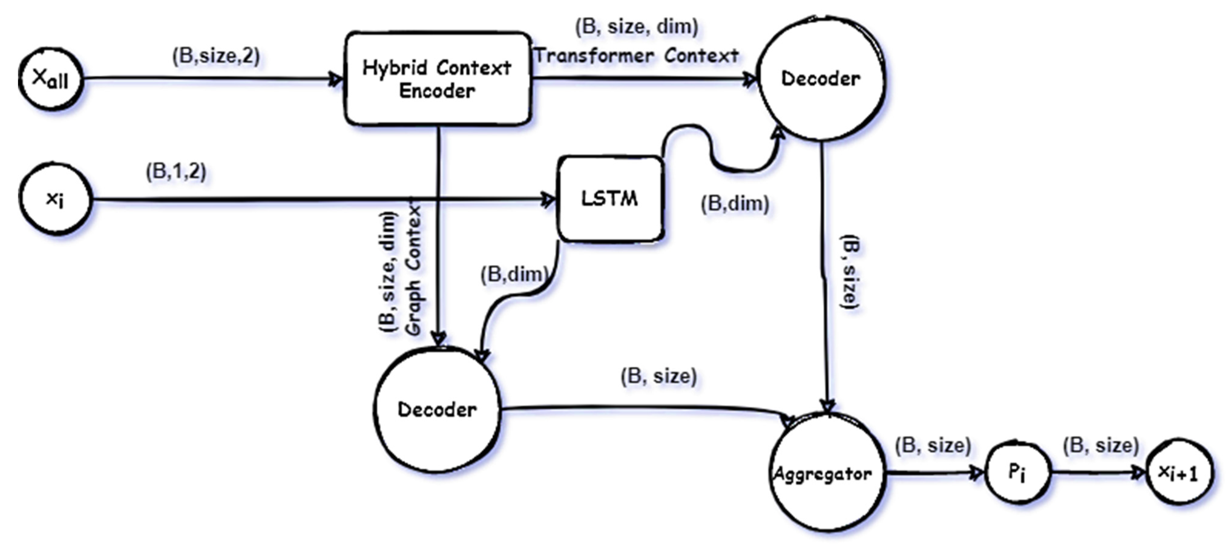
Figure 2.
Hybrid encoder.
Figure 2.
Hybrid encoder.
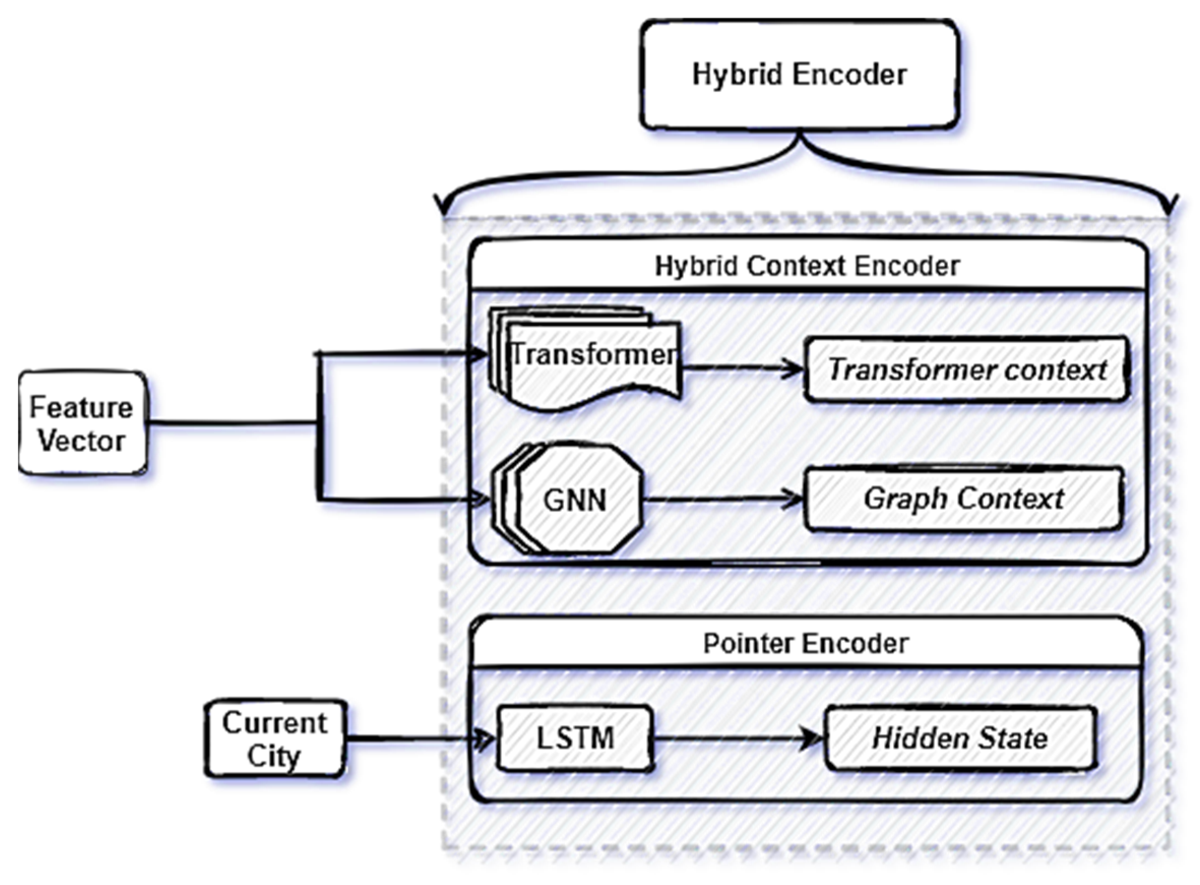
Figure 3.
Transformer’s Encoder used to encode the Feature Vector.
Figure 3.
Transformer’s Encoder used to encode the Feature Vector.
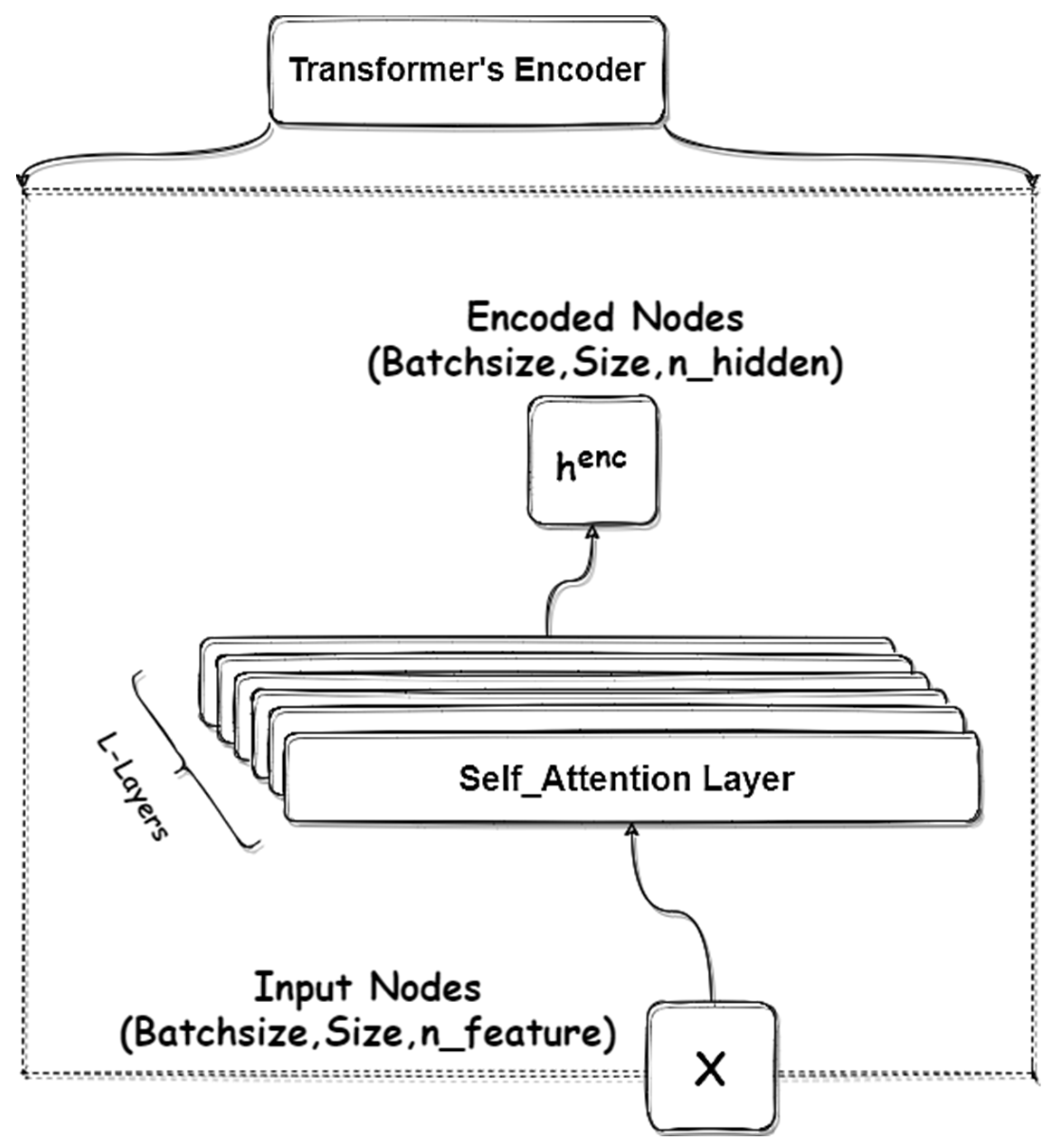
Figure 4.
Sample tours TWTSP20, TWTSP50 and TWTSP100 solved by HPN the cost included the total tour distance plus any time wait each point labeled with its time window (Entrance, Leaving) on 2D space on the left. On the right, plotting the x and y axes for the coordinates of the point and the z axis for the available time window for that point.
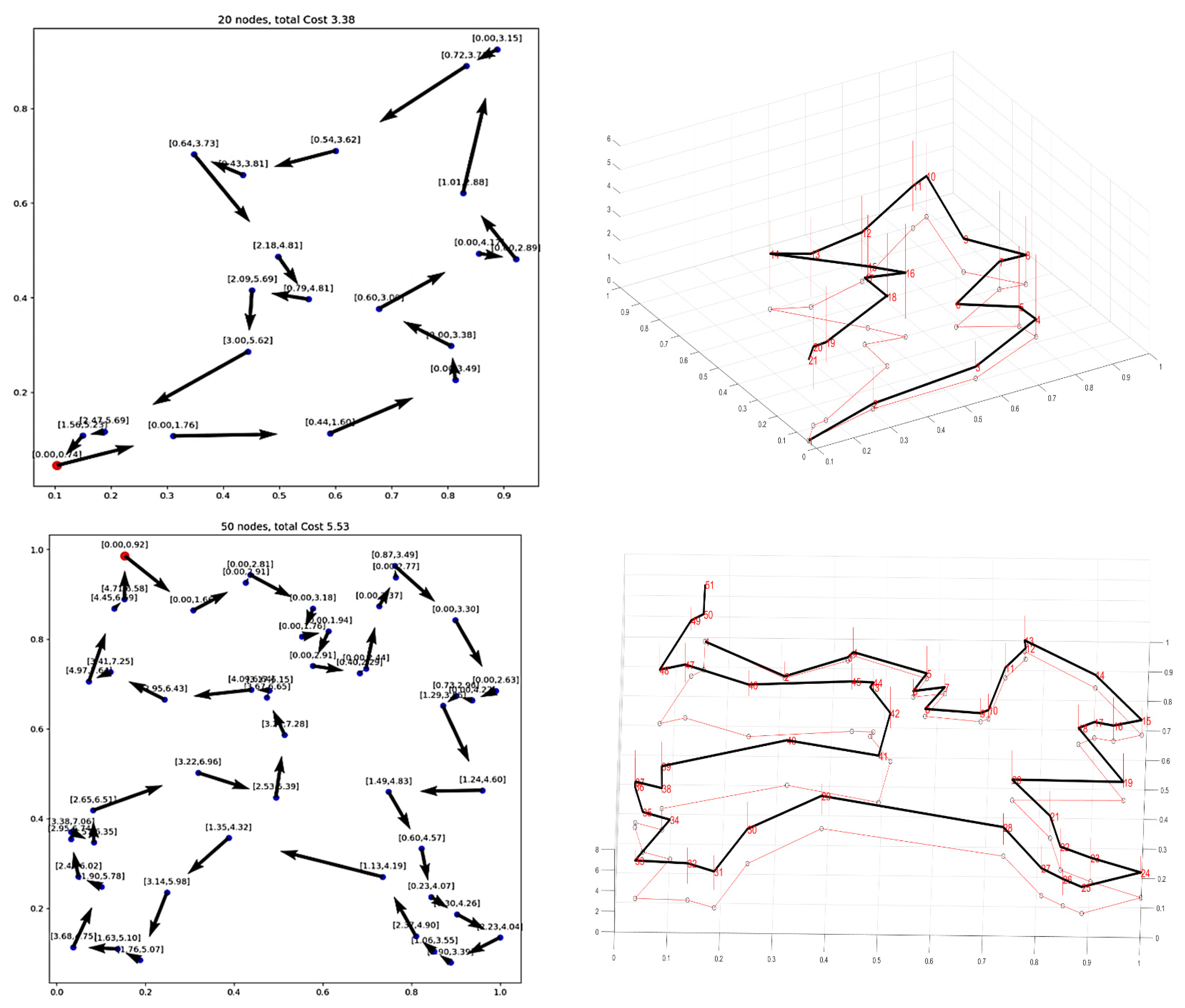
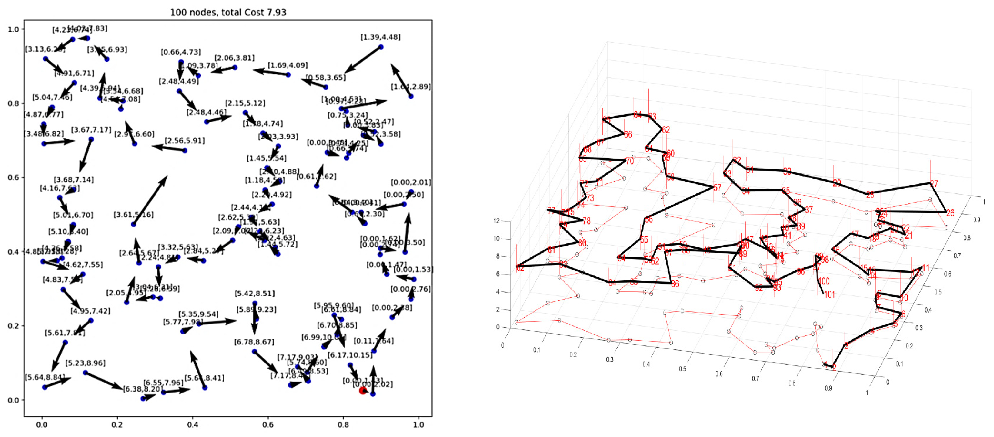
Figure 5.
Training performance for TWTSP20 with variable expected time window where the left panel shows the Actor performance, and the right panel shows the critic performance.
Figure 5.
Training performance for TWTSP20 with variable expected time window where the left panel shows the Actor performance, and the right panel shows the critic performance.
Table 1.
Mathematical terms for the TSPTW.
Table 1.
Mathematical terms for the TSPTW.
|
N |
Set of Nodes that Needs Service
{ 1 } |
|---|---|
|
N |
Set of all nodes in the network
{ 0 } |
|
N |
Set of all nodes that the salesman can depart
{ 0 } |
|
N |
Set of all nodes that the salesman can visit
{ 1 } |
|
t |
The time at the witch the salesman service node
i |
|
e |
The earliest time the salesman can service node
i |
|
l |
The latest time the salesman can arrive at node
i |
Table 2.
Hyperparameters used for training.
Table 2.
Hyperparameters used for training.
| Parameter | Value | Parameter | Value |
|---|---|---|---|
| Graph Embedding layer | 3 | Learning rate | 1 × 10⁻⁴ |
| Transformer Encoder | 6 | Batch size | 512 |
| Feed-forward dim | 512 | Training steps | 2500 |
| Optimizer | Adam | Tanh clipping | 10 |
| Epochs | 100 | Time Windows Expectation | 1 |
Table 3.
Illustration of the simulated data generation.
Table 3.
Illustration of the simulated data generation.
| #Algorithm 1 Data Simulation |
|---|
| 1: Input: pre-trained model for TSP, batch size B, problem size |
| 2: InputData = RandomInstance (B, size, 2) #Random generate TSP points
( x ) Features |
| 3: X = pre_trainedModel(InputData) #Solve the points using pre-trained model, X is a tensor |
| 4: PrevCities = FirstCities #contains the pre-trained model’s solution |
| 5: for t = 1,…, size do: |
| 6: current cities = X[t] #Pick the current city |
| 7: cur_time ← EuclideanDistance(current_cities, PrevCities) #Caluclate the Euc Distance |
| 8: X[:,t,2] ← max(0,(cur_time − 2 ∗ RandomNumber)) #Entrance Time |
| 9: X[:,t,3] ← cur_time + 2 ∗ RandomNumber + 1 #Leaving Time |
| 10: end for |
| 11: Shuffle(X) |
Table 4.
Results for TSPTW 20-50-100. Obj: objective of TSPTW. Time: the running time of the algorithms. Feasible %: the percentage of instances that have feasible solutions by the algorithm. All results are averaged from 10K instances.
Table 4.
Results for TSPTW 20-50-100. Obj: objective of TSPTW. Time: the running time of the algorithms. Feasible %: the percentage of instances that have feasible solutions by the algorithm. All results are averaged from 10K instances.
| TWTSP20 | TWTSP50 | TWTSP100 | |||||||
|---|---|---|---|---|---|---|---|---|---|
| Method | Obj | Time | Feasible% | Obj | Time | Feasible% | Obj | Time | Feasible% |
| OR-Tools (Savings) | 4.045 | 121 s | 72.06% | 6.251 | 1120 s | 70.21% | |||
| ACO | 4.655 | 204 s | 62.10% | 8.136 | 1493 s | 61.52% | |||
| GPN Greedy | 3.871 | 1 s | 99.7% | 5.95 | 3 s | 99.97% | 9.78 | 8 s | 32.8% |
| HPN Greedy | 3.867 | 1 s | 100% | 5.86 | 4 s | 100% | 8.32 | 12 s | 99.97% |
Table 5.
Total cost, time and feasible % metrics of the trained models versus the testing dataset generated using different expected time window width.
Table 5.
Total cost, time and feasible % metrics of the trained models versus the testing dataset generated using different expected time window width.
| NET1 (E(WT)) = ½ | NET2 (E(WT)) = 1 | NET3 (E(WT)) = 2 | NET4 (E(WT)) = 4 | |||||||||
|---|---|---|---|---|---|---|---|---|---|---|---|---|
| Cost | Wait | Acc | Cost | Wait | Acc | Cost | Wait | Acc | Cost | Wait | Acc | |
|
E = ½ |
3.89 | 0.003 | 99.99% | 3.89 | 0.002 | 99.8 | 3.90 | 0.003 | 99.62% | 4.2 | 0.001 | 85.5% |
|
E ( = 1 |
3.897 | 0.004 | 100% | 3.88 | 0.002 | 100% | 3.875 | 0.002 | 100% | 4.04 | 0.008 | 99.51% |
|
E ( = 2 |
4.14 | 0.009 | 100% | 3.93 | 0.005 | 100% | 3.858 | 0.001 | 100% | 3.91 | 0.003 | 100% |
|
E ( = 4 |
4.67 | 0.0113 | 100% | 4.39 | 0.013 | 100% | 3.985 | 0.009 | 100% | 3.836 | 0.0008 | 100% |
Table 6.
Evaluation performance for both Adam and Adam W, Cost indicates to the total cost for the tour which is the total tour length plus the total time wait.
Table 6.
Evaluation performance for both Adam and Adam W, Cost indicates to the total cost for the tour which is the total tour length plus the total time wait.
| Type of Data | NET1 AdamW | NET2 Adam | ||||
|---|---|---|---|---|---|---|
| Data-Variable-Exp | Cost | Acc | Wait | Cost | Acc | Wait |
|
E ( = ½ |
3.875 | 100% | 0.0037 | 3.877 | 100% | 0.003 |
|
E ( = 1 |
3.89 | 99.14% | 0.0022 | 3.90 | 98.76% | 0.0019 |
|
E ( = 2 |
3.885 | 99.89% | 0.002 | 3.887 | 99.97% | 0.0019 |
|
E ( = 4 |
3.88 | 99.98% | 0.003 | 3.876 | 100% | 0.003 |
|
E ( = 8 |
3.875 | 100% | 0.005 | 3.887 | 100% | 0.007 |
|
E ( = 16 |
4.086 | 100% | 0.008 | 3.99 | 100% | 0.03 |
|
Publisher’s Note: MDPI stays neutral with regard to jurisdictional claims in published maps and institutional affiliations. |
We present a new solution approach for the Time Dependent Traveling Salesman Prob- lem with Time Windows. This problem considers a salesman who departs from his home, has to visit a number of cities within a pre-determined period of time, and then returns home. The problem allows for travel times that can depend on the time of departure. The solution approach is based on an integer programming formulation of the problem on a time expanded network, as doing so enables time dependencies to be embedded in the definition of the network. However, as such a time expanded network (and thus the integer programming formulation) can rapidly become prohibitively large, the solution approach employs a dynamic discretization discovery framework, which has been effective in other contexts. Our computational results indicate that the so- lution approach outperforms the best-known methods on benchmark instances and is robust with respect to instance parameters.
Article
Download
View Solving Time Dependent Traveling Salesman Problems with Time Windows